How to Shiny

What is Shiny? (Recap)

An R package that allows for more functionality within the software
Allows users to create interactive web pages for data science

How to Install Shiny

Since Shiny is not in base R, you will need to install it…

Install package:

install.packages("shiny")

Load package:

library(shiny)

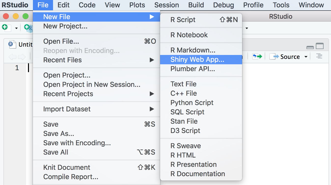
Getting Started

File > New File > Shiny Web App

Application type: Single File is best (easier to keep track of code)

Example of a Shiny App

Iris k-means clustering

Sidebar and Plot (UI)

ui <- pageWithSidebar(
  headerPanel('Iris k-means clustering'), ## Title
  sidebarPanel( ## Creates a panel on the left side of screen
    selectInput('xcol', 'X Variable', vars), 
    ## Dropdown for picking X variable
    selectInput('ycol', 'Y Variable', vars, selected = vars[[2]]), 
    ## Dropdown for picking Y variable
    numericInput('clusters', 'Cluster count', 3, min = 1, max = 9) 
    ## Option to pick number of clusters
  ),
  mainPanel(
    plotOutput('plot1') ## Names your output variable
  )
)

Remember, we need to do our server-side code or this will not work!

Back-end Code (Server)

server <- function(input, output, session) {

  ## Combine the selected variables into a new data frame
  selectedData <- reactive({
    iris[, c(input$xcol, input$ycol)]
  ## selectedData is reactive!
  ## Contains only selected X and Y variables
  })

  clusters <- reactive({
    kmeans(selectedData(), input$clusters)
  })
  ## Performs clustering based on number of user selected clusters

Back-end Code (Server)

  output$plot1 <- renderPlot({
    palette(c("#E41A1C", "#377EB8", "#4DAF4A", "#984EA3",
      "#FF7F00", "#FFFF33", "#A65628", "#F781BF", "#999999"))
      ## Renders the plot using custom colors

    par(mar = c(5.1, 4.1, 0, 1))
    plot(selectedData(),
         col = clusters()$cluster,
         pch = 20, cex = 3)
    points(clusters()$centers, pch = 4, cex = 4, lwd = 4)
  })
  
  ## Plots points 
  ## You will use ggplot instead of this syntax!
}

Run the App!

shinyApp(ui, server)

Since you will be using a combined file, you must run this command to run the app.

Creating your App

Load your Packages (I used a lot - don’t need all to begin!)

## Important packages
library(ggplot2)
library(shiny)
library(dplyr)
library(tidyr)
library(ggplotlyExtra) ## Convert ggplot2 plots to plotly
library(plotly)

library(bslib) ## Extra functionality within Shiny
library(shinyWidgets) ## Extra functionality within Shiny
library(gghalves)
library(ggforce)
library(ggdist)
library(shinycssloaders) ## Adds loading wheel to outputs
library(shinytitle) ## Gives your page a name on browser

Creating your App cont.

Load and Clean Data

data <- read.csv("health_status_data.csv")
## Load csv as "data" variable

data <- data %>% select(-SAMPLE1, -SAMPLE2, -SAMPLE3, -SAMPLE4, -SAMPLE5,-RI_1, -RI_2, -RI_3, -RI_4, -RI_5, -RI_6, -RI_7, -RI_8)
## Selecting all columns EXCEPT the ones above

data <- data %>% mutate(  ## this is a pipe (%>%)
  
  SEX = case_when(SEX == 0 ~ "Male",
                  SEX == 1 ~ "Female",
                  SEX == 2 ~ "Intersex",
                  SEX == 3 ~ "Other")
                      )
                      
## data <- data means making our changes PERMANENT

Keep variable names concise and easily recognizable!

Creating your App cont.

Create UI and Server Code

Using Plotly for graphs is often better because of its extra functionality.

## UI:
## Use plotlyOutput() instead of plotOutput()

## Server:
## Wrap your ggplot code within ggplotly(),
## ***put actual ggplot2 code in placeholder***

ggplotly(***ggplot2 code***)


## Use renderPlotly({}) instead of renderPlot({})

Creating your App cont.

Create UI and Server Code

Same with DT for datatables.

## UI:
## Use DT::dataTableOutput() instead of tableOutput()

## Server:
## Use DT::renderDataTable({}) instead of renderTable({})

Links to Other Resources

Previous Shiny Presentation

Shiny Cheatsheet

Mastering Shiny