Back to Article
Analysis of Variance (ANOVA)
Download Source

Analysis of Variance (ANOVA)

for Each Zero-Sum Belief Items using Political Party Affiliation

Authors
Affiliations

Aashia Khan

Binghamton University

Zihan Hei

Binghamton University

Jeff John

Binghamton University

Shane McCarty

Binghamton University

Promote Care & Prevent Harm

Published

February 15, 2026

Abstract

Background: Zero-sum beliefs—the perception that one group’s gains necessarily result in another group’s losses—are important predictors of political attitudes. However, the referents for zero-sum beliefs as economic or social identity remain underexplored in relation to political ideology, party affiliation, and voting behavior in contemporary elections.

Method: We conducted a comprehensive analysis examining three dimensions of zero-sum beliefs (general, economic, and social identity). Using Kruskal-Wallis tests on eleven zero-sum beliefs, we investigated how political party affiliation and racial/ethnic identity influenced endorsement of zero-sum beliefs across multiple domains. Subsequently, we examined whether these zero-sum belief patterns predicted self-reported voting for Donald Trump versus Kamala Harris in the 2024 presidential election.

Results: Political party affiliation was a significant predictor for all eight zero-sum social identity beliefs, but none of the economic or general beliefs. Republican voters and certain racial/ethnic groups demonstrated higher endorsement of zero-sum social identity beliefs. A logistic regression shows that after controlling for political ideology, a composite of zero-sum social identity beliefs explains voting behavior in the 2024 presidential election, with stronger zero-sum social identity thinking associated with Trump support and lower zero-sum social identity beliefs predicting Harris support. Other sociodemographic factors and zero-sum economic thinking were not significant predictors.

Discussion: Zero-sum social identity beliefs may represent a competitive core belief underlying contemporary political party affiliation and candidate preference. These findings affirm prior work that zero-sum thinking about economics differ from social identities, with similar levels of agreement on zero-sum economic beliefs across political parties but significantly different levels of agreement on zero-sum social identity beliefs by party affiliation. To the best of our knowledge, this study is the first to show that zero-sum thinking about social identities predicts voter preference in the 2024 election. Ultimately, future work needs to examine how to reduce zero-sum social identity thinking.

Keywords

zero sum beliefs, social identities, political affiliation, racial identity

Introduction

Political Realignment (SM)

Zero-Sum Beliefs Regarding Game, Economic, and Social Identities (AK, JJ)

Zero-Sum Beliefs and Political Party (AK)

Zero-Sum Beliefs and Racial Identity (JJ)

Zero-Sum Beliefs and Voter Behavior (AK)

Methods

Study Participants (AK)

More than fifty-five thousand people who are active on the Prolific platform were eligible to complete a 45-minute health beliefs survey with measures on various beliefs associated with politics and health. Using a quota sample by sex (50% male/ 50% female), political affiliation (33% Republican, 33% Democrat, and 34% Independent), and race/ethnicity (White 40%, Black 20%, Asian 20%, Mixed 10%, and Other 10%), Prolific recruited one hundred and twenty-five people to complete the survey.

Measures (AK)

This needs updating …

Respondents were asked to report their gender (selections: Girl or woman, boy or man, nonbinary/genderfluid/genderqueer, I am not sure/questioning), race (selections: American Indian or Alaska Native, Asian, Black or African American, Hispanic or Latine, Middle Eastern or North African, Native Hawaiian/Pacific Islander, White), social status (selections: Lowest 1- Highest 10), and political beliefs (selections: far left/leftist, very liberal, liberal, moderate, conservative, very conservative, alt-right/far-right). Respondents were asked to report their level of agreement using a likert scale (1: Strongly Disbelieve, 2: Disbelieve, 3: Somewhat Disbelieve, 4: Neither, 5: Somewhat Believe, 6: Believe, 7: Strongly Believe) with X number of statements. - political affiliation/party - political ideology/beliefs - gender - education - social class - racial identity - 2024 voting behavior

Analysis Plan (ZH)

Two-way Analysis of Variance (ANOVA) were run on 11 zero-sum beliefs ( ZEROSUM_ ) – including X economic zero-sum and X social identity zero-sum beliefs – using the factors of political affiliation ( POLITICALPARTY ) and racial/ethnic identity ( RACIALIDENTITY.4 ).

An explanatory logistic regression was conducted to classy voter’s preference for Donald Trump (1) vs. Kamala Harris (0) ( TRUMPVOTE ) using GENDER_MALE, RACE_WHITE, EDUCATION_HIGH, SOCIALCLASS, POLITICALBELIEFS, ZEROSUM_IDENTITY, ZEROSUM_ECONOMIC, and ZEROSUM_1.

ZH: Additionally, we used tidymodels package in R to classify using a predictive model. Using an integrative modeling approach, we provide an explanatory and predictive model for classifying voter preferences.

Results

In [1]:
Show the code

# Load necessary libraries
library(ggplot2)
library(plotly)

Attaching package: 'plotly'
The following object is masked from 'package:ggplot2':

    last_plot
The following object is masked from 'package:stats':

    filter
The following object is masked from 'package:graphics':

    layout
Show the code

library(dplyr)

Attaching package: 'dplyr'
The following objects are masked from 'package:stats':

    filter, lag
The following objects are masked from 'package:base':

    intersect, setdiff, setequal, union
Show the code

library(tidyr)
library(ggrain)  
Registered S3 methods overwritten by 'ggpp':
  method                  from   
  heightDetails.titleGrob ggplot2
  widthDetails.titleGrob  ggplot2
Show the code

library(rmarkdown)
library(readr)
library(patchwork)
library(codebookr)
library(dplyr, warn.conflicts = FALSE)
library(haven)
library(codebook)

Attaching package: 'codebook'
The following object is masked from 'package:codebookr':

    codebook
Show the code

library(rempsyc)
Suggested APA citation: Thériault, R. (2023). rempsyc: Convenience functions for psychology. 
Journal of Open Source Software, 8(87), 5466. https://doi.org/10.21105/joss.05466
Show the code

library(car)
Loading required package: carData

Attaching package: 'car'
The following object is masked from 'package:dplyr':

    recode
Show the code

library(knitr)
library(broom)
library(ggdist)
library(patchwork)
library(car)
library(dataMaid)

Attaching package: 'dataMaid'
The following object is masked from 'package:rmarkdown':

    render
The following object is masked from 'package:dplyr':

    summarize
Show the code

library(devtools)
Loading required package: usethis

Attaching package: 'devtools'
The following object is masked from 'package:dataMaid':

    check
Show the code

library(MBESS)
library(apaTables)
library(ggpubr)
library(psych)

Attaching package: 'psych'
The following object is masked from 'package:MBESS':

    cor2cov
The following object is masked from 'package:car':

    logit
The following object is masked from 'package:codebook':

    bfi
The following objects are masked from 'package:ggplot2':

    %+%, alpha
Show the code

library(forcats)
library(corrplot)
corrplot 0.95 loaded
In [2]:
Show the code
select_data <- read.csv("/cloud/project/data/select_data.csv")
In [3]:
Show the code

table(select_data$ETHNICITY)

      Asian       Black Mixed/Other       White 
         24          25          25          48 
Show the code

## notice that the groups are unequal which is a problem for the ANOVA.
## TO DO: consider whether we should do a non-parametric approach

# SOURCE FOR DUMMY CODE
## https://stats.oarc.ucla.edu/other/mult-pkg/faq/general/faqwhat-is-dummy-coding/
## https://www.nathanwhudson.com/courses/methods/resources/10.%20Dummy%20Coding.pdf
## can you find an R specific example? 
In [4]:
Show the code

party_colors <- c("Democrat" = "#0015BC", "Republican" = "#E9141D", "Independent" = "#732C7B")

Factors Associated with Zero-Sum Beliefs

Zero Sum 1

In [5]:
Show the code

library(dplyr)

## We group by both political party and racial identity to explore whether attitudes about zero-sum beliefs differ across these two demographic factors.
## Then, we summarize the data using dplyr's `summarise()` to calculate:
## - mean of ZEROSUM_1 (agreement with zero-sum beliefs)
## - standard error (SE) of the mean, which reflects the variability in responses

group_stats_1 <- select_data %>%
  group_by(POLITICALPARTY, RACIALIDENTITY.4) %>%
  summarise(
    mean_ZEROSUM_1 = mean(ZEROSUM_1, na.rm = TRUE),  # average score for each group
    se = sd(ZEROSUM_1, na.rm = TRUE) / sqrt(n()),    # standard error for error bars
    .groups = 'drop'   # ungroup for downstream operations
  )

# Quick check of the output's structure and first few rows
str(group_stats_1)
tibble [12 × 4] (S3: tbl_df/tbl/data.frame)
 $ POLITICALPARTY  : chr [1:12] "Democrat" "Democrat" "Democrat" "Democrat" ...
 $ RACIALIDENTITY.4: chr [1:12] "Asian" "Black" "Mixed/Other" "White" ...
 $ mean_ZEROSUM_1  : num [1:12] 4.25 4.5 3 3.88 3.12 ...
 $ se              : num [1:12] 0.491 0.5 0.5 0.514 0.549 ...
Show the code

head(group_stats_1)
# A tibble: 6 × 4
  POLITICALPARTY RACIALIDENTITY.4 mean_ZEROSUM_1    se
  <chr>          <chr>                     <dbl> <dbl>
1 Democrat       Asian                      4.25 0.491
2 Democrat       Black                      4.5  0.5  
3 Democrat       Mixed/Other                3    0.5  
4 Democrat       White                      3.88 0.514
5 Independent    Asian                      3.12 0.549
6 Independent    Black                      3.75 0.75 
In [6]:
Show the code

## This plot visualizes how different political and racial groups scored on the ZEROSUM_1 scale
## We use a point-range plot to show:
##  - the group mean (point)
##  - variability (standard error bars above and below the mean)

## The color of each point reflects the racial identity of respondents

zesty_four <- c("#E69F00", "#009E73", "#999999", "#CC79A7")  # custom color palette

plot.zerosum1 <- ggplot(group_stats_1, aes(POLITICALPARTY, mean_ZEROSUM_1)) +
  geom_pointrange(aes(
      color = RACIALIDENTITY.4,
      ymin = mean_ZEROSUM_1 - se,  # lower bound of SE
      ymax = mean_ZEROSUM_1 + se   # upper bound of SE
    ),
    position = position_dodge(0.3)) +
  theme_bw() +
  labs(
    title = "Life is so devised that when somebody gains, others have to lose.",
    x = "Political Affiliation",
    y = "Agreement with Zero Sum Beliefs",
    color = "RACIALIDENTITY.4"
  ) +
  theme(
    plot.title = element_text(size = 12, face = "bold", hjust = 0.5),
    axis.title = element_text(size = 10),
    axis.text = element_text(size = 8),
    legend.title = element_text(size = 10),
    legend.text = element_text(size = 8)
  ) +
  scale_y_continuous(
    breaks = 1:7,
    labels = c("1: Strongly Disbelieve", "2: Disbelieve", "3: Somewhat Disbelieve",
               "4: Neither", "5: Somewhat Believe", "6: Believe", "7: Strongly Believe"),
    limits = c(1, 7)
  ) +
  scale_color_manual(values = zesty_four)

# Print and save the plot for documentation
print(plot.zerosum1)

Show the code

ggsave("plot1:gain-lose.png", plot = plot.zerosum1, width = 10, height = 8, dpi = 300)
In [7]:
Show the code

## This chunk computes the 95% confidence intervals (CIs) for the mean ZEROSUM_1 score by political party.
## Unlike SE, a CI gives a sense of the range in which the true population mean likely falls.

group_stats_1_avg <- select_data %>%
  group_by(POLITICALPARTY) %>%
  summarise(
    mean_ZEROSUM_1 = mean(ZEROSUM_1, na.rm = TRUE),
    se = sd(ZEROSUM_1, na.rm = TRUE) / sqrt(n()),  # standard error
    n = n(),
    .groups = 'drop'
  ) %>%
  mutate(
    # Calculate t-critical value for 95% CI using the t-distribution
    t_value = qt(0.975, df = n - 1),
    ci_lower = mean_ZEROSUM_1 - t_value * se,
    ci_upper = mean_ZEROSUM_1 + t_value * se
  )

## These statistics will be used for overlaying on the raincloud plot later
In [8]:
Show the code

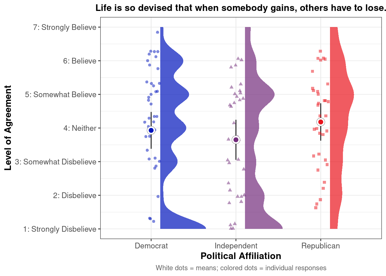
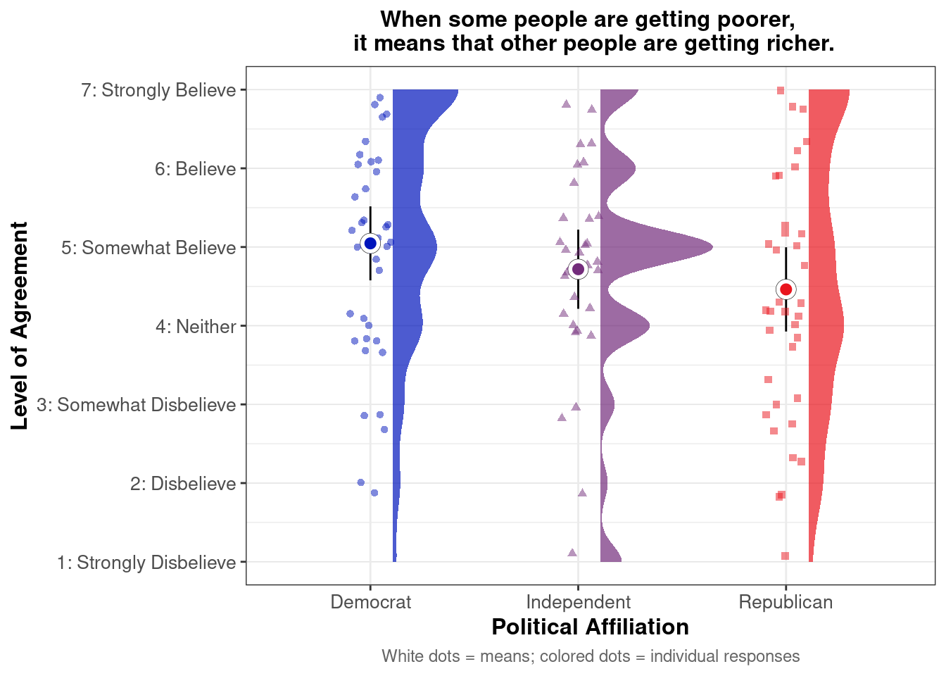
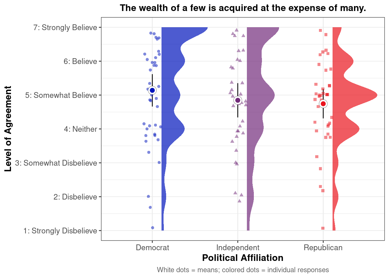
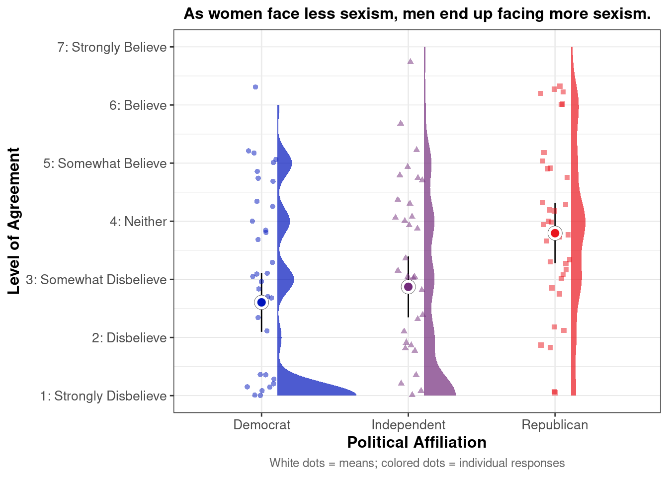
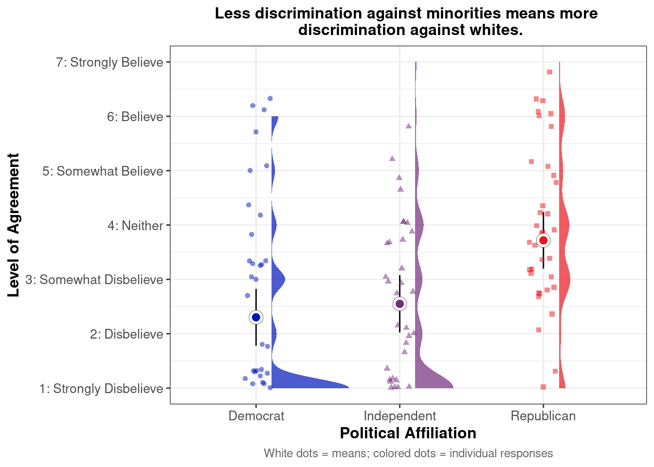
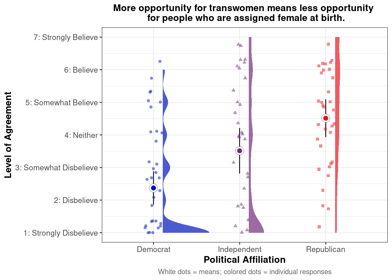
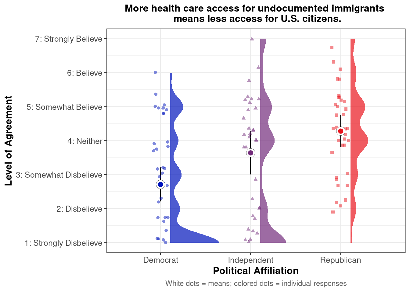
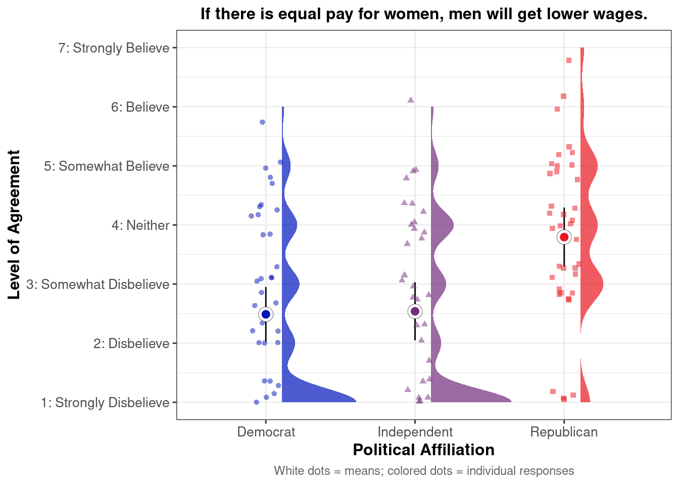
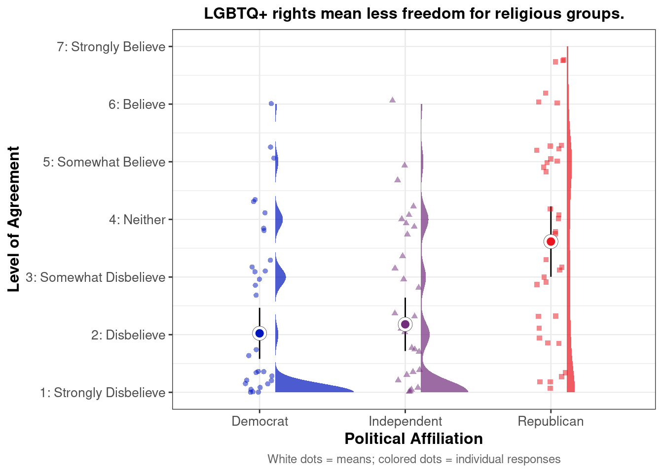
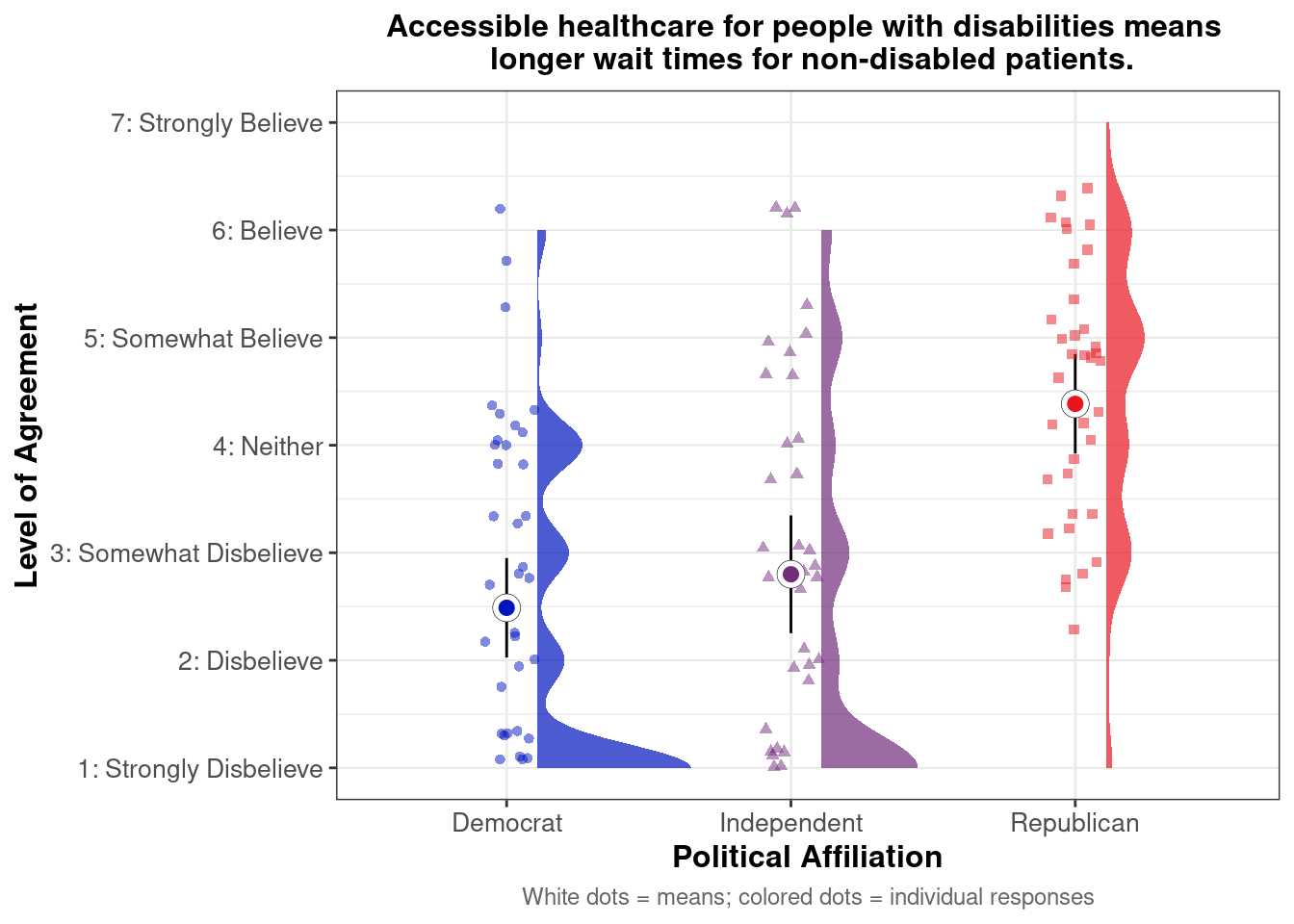
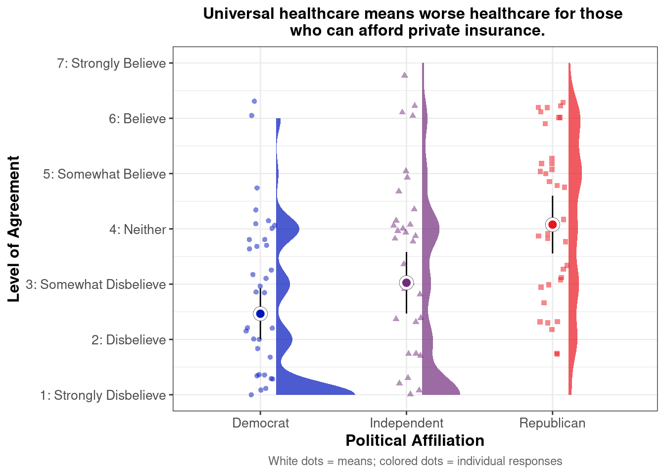
## This chunk creates a "raincloud plot" to visualize the distribution of ZEROSUM_1 scores by political party. 
## Raincloud plots combine density shapes, raw data points, and summary stats (mean + CI).

plot.zerosum1_raincloud <- select_data %>%
  filter(!is.na(ZEROSUM_1), !is.na(POLITICALPARTY)) %>%
  ggplot(aes(x = POLITICALPARTY, y = ZEROSUM_1, fill = POLITICALPARTY, color = POLITICALPARTY)) +

## Half-eye density shows the distribution shape (like a smoothed histogram).
  stat_halfeye(
    adjust = 0.5,         
    width = 0.6,          
    .width = 0,           
    justification = -0.2, 
    point_colour = NA,
    alpha = 0.7           
  ) +

## Add 95% confidence intervals from earlier calculations
  geom_pointrange(
    data = group_stats_1_avg,
    aes(
      x = POLITICALPARTY,
      y = mean_ZEROSUM_1,
      ymin = ci_lower,
      ymax = ci_upper
    ),
    color = "black",      
    size = 0.9,
    shape = 21,
    fill = "white",
    stroke = 1.2,
    inherit.aes = FALSE   
  ) +

## Add jittered raw data points (each dot = individual response)
  geom_point(
    aes(shape = POLITICALPARTY),
    size = 1.5,
    alpha = 0.5,
    position = position_jitter(
      seed = 1, width = 0.1  # keeps jitter reproducible
    )
  ) +

## Overlay group means as white dots
  stat_summary(
    fun = mean,
    geom = "point",
    size = 3,
    color = "white",
    stroke = 1.5,
    shape = 21
  ) +

## Color palette and theming
  scale_fill_manual(values = party_colors) +
  scale_color_manual(values = party_colors) +
  theme_bw() +
  labs(
    title = "Life is so devised that when somebody gains, others have to lose.",
    x = "Political Affiliation",
    y = "Level of Agreement",
    caption = "White dots = means; colored dots = individual responses"
  ) +
  theme(
    plot.title = element_text(size = 12, face = "bold", hjust = 0.5),
    plot.caption = element_text(size = 9, color = "gray40", hjust = 0.5),
    axis.title = element_text(size = 12, face = "bold"),
    axis.text = element_text(size = 10),
    legend.position = "none",
    panel.grid.major.y = element_line(color = "gray90", linewidth = 0.3)
  ) +
  
## Match axis scale to Likert-style labels for interpretation
  scale_y_continuous(
    breaks = 1:7,
    labels = c("1: Strongly Disbelieve", 
               "2: Disbelieve", 
               "3: Somewhat Disbelieve", 
               "4: Neither", 
               "5: Somewhat Believe", 
               "6: Believe", 
               "7: Strongly Believe"),
    limits = c(1, 7)
  )

## Show the final plot
plot.zerosum1_raincloud
Warning: Removed 16 rows containing missing values or values outside the scale range
(`geom_point()`).

Inconsistent ANOVA results

aov() function is used for NO interactions, but we have an interaction of POLITICALPARTY * RACIALIDENTITY.4therefore, we should use the newer package within the linear model lm function using type = 2.

THIS IS THE CODE BLOCK TO USE THROUGHOUT THE REPORT

In [9]:
Show the code

## two way ANOVA using  
library(car)
model.ZEROSUM_1.PE <- lm(ZEROSUM_1 ~ POLITICALPARTY * RACIALIDENTITY.4, data = select_data)
Anova(model.ZEROSUM_1.PE, type = 2)
Anova Table (Type II tests)

Response: ZEROSUM_1
                                Sum Sq  Df F value Pr(>F)
POLITICALPARTY                    4.81   2  0.7316 0.4835
RACIALIDENTITY.4                  6.63   3  0.6730 0.5704
POLITICALPARTY:RACIALIDENTITY.4  11.55   6  0.5860 0.7409
Residuals                       361.45 110               
Show the code

## There is no statistically significant difference in ZEROSUM_1 scores between political parties, ethnicities, or their interaction.
In [10]:
Show the code

# Two-way ANOVA
model.ZEROSUM_1.PE <- lm(ZEROSUM_1 ~ POLITICALPARTY * RACIALIDENTITY.4, data = select_data)

anova_df <- as.data.frame(Anova(model.ZEROSUM_1.PE, type = 2))%>%
  tibble::rownames_to_column(var = "Predictor")
names(anova_df)[names(anova_df) == "Pr(>F)"] <- "p"

# APA format
nice_table(anova_df, 
           title = c("Table 1", "ZeroSum_1 ANOVA Table"), 
           highlight = 0.05, 
           stars = TRUE)

Table 1

ZeroSum_1 ANOVA Table

Predictor

Sum Sq

Df

F value

p

POLITICALPARTY

4.81

2.00

0.73

.483

RACIALIDENTITY.4

6.63

3.00

0.67

.570

POLITICALPARTY × RACIALIDENTITY.4

11.55

6.00

0.59

.741

Residuals

361.45

110.00

Show the code

## There is no statistically significant difference in ZEROSUM_1 scores between political parties, ethnicities, or their interaction.
In [11]:
Show the code

plot(model.ZEROSUM_1.PE)  # diagnostic plots

Show the code

shapiro.test(residuals(model.ZEROSUM_1.PE))  # normality test

    Shapiro-Wilk normality test

data:  residuals(model.ZEROSUM_1.PE)
W = 0.95307, p-value = 0.0003223
In [12]:
Show the code

# Check how bad the non-normality is
hist(residuals(model.ZEROSUM_1.PE))

Show the code

# check: for normal distribution
# results: not normal, but it's close (and likely would be with larger sample size)
# interpretation: this is okay

qqnorm(residuals(model.ZEROSUM_1.PE))
# check: points should fall near the diagonal line 
# results: potential outliers at the extremes

qqline(residuals(model.ZEROSUM_1.PE))

Show the code

# check: for outliers
# results: no outliers
# interpretation: even though we violate assumptions previously, there are not outliers to drop to improve interpretation
In [13]:
Show the code

boxplot(residuals(model.ZEROSUM_1.PE))

Show the code

# check: for outliers
# results: no outliers
# interpretation: even though we violate assumptions previously, there are not outliers to drop to improve interpretation

## overall: the visual inspection across the previous plots suggests we are okay to move forward with the ANOVA test, but must report the shapiro.test results here. 

Zero Sum 2

In [14]:
Show the code

library(dplyr)
group_stats_2 <- select_data %>%
  group_by(POLITICALPARTY, RACIALIDENTITY.4) %>%
  summarise(
    mean_ZEROSUM_2 = mean(ZEROSUM_2, na.rm = TRUE),
    se = sd(ZEROSUM_2, na.rm = TRUE) / sqrt(n()),
    .groups = 'drop'
  )

# Check the structure
str(group_stats_2)
tibble [12 × 4] (S3: tbl_df/tbl/data.frame)
 $ POLITICALPARTY  : chr [1:12] "Democrat" "Democrat" "Democrat" "Democrat" ...
 $ RACIALIDENTITY.4: chr [1:12] "Asian" "Black" "Mixed/Other" "White" ...
 $ mean_ZEROSUM_2  : num [1:12] 5.75 5.1 3.88 5.24 4 ...
 $ se              : num [1:12] 0.526 0.314 0.611 0.369 0.655 ...
Show the code

head(group_stats_2)
# A tibble: 6 × 4
  POLITICALPARTY RACIALIDENTITY.4 mean_ZEROSUM_2    se
  <chr>          <chr>                     <dbl> <dbl>
1 Democrat       Asian                      5.75 0.526
2 Democrat       Black                      5.1  0.314
3 Democrat       Mixed/Other                3.88 0.611
4 Democrat       White                      5.24 0.369
5 Independent    Asian                      4    0.655
6 Independent    Black                      3.71 0.699
In [15]:
Show the code

# Define the zesty_four palette
zesty_four <- c("#F5793A", "#A95AA1", "#85C0F9", "#0F2080") 

# Create the plot with pointrange
plot.zerosum2 <- ggplot(group_stats_2, 
                        aes(POLITICALPARTY, mean_ZEROSUM_2)) +
  geom_pointrange(aes(color = RACIALIDENTITY.4,
                      ymin = mean_ZEROSUM_2 - se,
                      # Use standard error instead of sd
                      ymax = mean_ZEROSUM_2 + se),
                      # Use standard error instead of sd
                      position = position_dodge(0.3)) +
  theme_bw() +
  labs(title = "When some people are getting poorer, \n it means that other people are getting richer.",
       x = "Political Affiliation",
       y = "Agreement with Zero Sum Beliefs",
       color = "RACIALIDENTITY.4") + 
  theme(
    plot.title = element_text(size = 12, face = "bold", hjust = 0.5),
    axis.title = element_text(size = 10),
    axis.text = element_text(size = 8),
    legend.title = element_text(size = 10),
    legend.text = element_text(size = 8)
  ) +
  scale_y_continuous(
    breaks = 1:7,
    labels = c("1: Strongly Disbelieve", 
               "2: Disbelieve", 
               "3: Somewhat Disbelieve", 
               "4: Neither", 
               "5: Somewhat Believe", 
               "6: Believe", 
               "7: Strongly Believe"),
    limits = c(1, 7)  # Set the y-axis limits to match the scale
  )+
  scale_color_manual(values = zesty_four)

# Print and save the plots
print(plot.zerosum2)

Show the code

ggsave("plot2:poor-rich.png", 
       plot = plot.zerosum2, 
       width = 10, 
       height = 8, 
       dpi = 300)
In [16]:
Show the code

# ZEROSUM_1 average score with 95% CI
group_stats_2_avg <- select_data %>%
  group_by(POLITICALPARTY) %>%
  summarise(
    mean_ZEROSUM_2 = mean(ZEROSUM_2, na.rm = TRUE),
    se = sd(ZEROSUM_2, na.rm = TRUE) / sqrt(n()),
    n = n(),
    .groups = 'drop'
  ) %>%
  mutate(
    # Calculate 95% confidence interval using t-distribution
    t_value = qt(0.975, df = n - 1),  # 95% CI, two-tailed
    ci_lower = mean_ZEROSUM_2 - t_value * se,
    ci_upper = mean_ZEROSUM_2 + t_value * se
  )
In [17]:
Show the code

library(ggdist)
library(patchwork)

plot.zerosum2_raincloud <- select_data %>%
  filter(!is.na(ZEROSUM_2), !is.na(POLITICALPARTY)) %>%
  ggplot(aes(x = POLITICALPARTY, y = ZEROSUM_2, fill = POLITICALPARTY, color = POLITICALPARTY)) +
  stat_halfeye(
    adjust = 0.5,
    width = 0.6,
    .width = 0,
    justification = -0.2,
    point_colour = NA,
    alpha = 0.7
  ) +
  geom_pointrange(
      data = group_stats_2_avg,
      aes(
        x = POLITICALPARTY,
        y = mean_ZEROSUM_2,
        ymin = ci_lower,
        ymax = ci_upper
      ),
      color = "black",
      size = 0.9,
      shape = 21,
      fill = "white",
      stroke = 1.2,
      inherit.aes = FALSE
    ) +
  geom_point(
    aes(shape = POLITICALPARTY),
    size = 1.5,
    alpha = 0.5,
    position = position_jitter(
      seed = 1, width = 0.1
    )
  ) +
  stat_summary(
    fun = mean,
    geom = "point",
    size = 3,
    color = "white",
    stroke = 1.5,
    shape = 21
  ) +
  scale_fill_manual(values = party_colors) +
  scale_color_manual(values = party_colors) +
  theme_bw() +
  labs(
    title = "When some people are getting poorer, \n it means that other people are getting richer.",
    x = "Political Affiliation",
    y = "Level of Agreement",
    caption = "White dots = means; colored dots = individual responses"
  ) +
  theme(
    plot.title = element_text(size = 12, face = "bold", hjust = 0.5),
    plot.caption = element_text(size = 9, color = "gray40", hjust = 0.5),
    axis.title = element_text(size = 12, face = "bold"),
    axis.text = element_text(size = 10),
    legend.position = "none",
    panel.grid.major.y = element_line(color = "gray90", linewidth = 0.3)  # Fixed
  ) +
  scale_y_continuous(
    breaks = 1:7,
    labels = c("1: Strongly Disbelieve", 
               "2: Disbelieve", 
               "3: Somewhat Disbelieve", 
               "4: Neither", 
               "5: Somewhat Believe", 
               "6: Believe", 
               "7: Strongly Believe"),
    limits = c(1, 7) 
  )
plot.zerosum2_raincloud
Warning: Removed 14 rows containing missing values or values outside the scale range
(`geom_point()`).

In [18]:
Show the code

# Two-way ANOVA
model.ZEROSUM_2.PE <- lm(ZEROSUM_2 ~ POLITICALPARTY * RACIALIDENTITY.4, data = select_data)
Anova(model.ZEROSUM_2.PE)
Anova Table (Type II tests)

Response: ZEROSUM_2
                                 Sum Sq  Df F value  Pr(>F)  
POLITICALPARTY                    7.706   2  1.7140 0.18497  
RACIALIDENTITY.4                 26.379   3  3.9113 0.01072 *
POLITICALPARTY:RACIALIDENTITY.4  24.078   6  1.7851 0.10874  
Residuals                       245.040 109                  
---
Signif. codes:  0 '***' 0.001 '**' 0.01 '*' 0.05 '.' 0.1 ' ' 1
Show the code

## There is no statistically significant difference in ZEROSUM_2 scores between political parties, ethnicities, or their interaction.
In [19]:
Show the code

# Two-way ANOVA
model.ZEROSUM_2.PE <- lm(ZEROSUM_2 ~ POLITICALPARTY * RACIALIDENTITY.4, data = select_data)

anova_df <- as.data.frame(Anova(model.ZEROSUM_2.PE, type = 2))%>%
  tibble::rownames_to_column(var = "Predictor")
names(anova_df)[names(anova_df) == "Pr(>F)"] <- "p"

# APA format
nice_table(anova_df, 
           title = c("Table 2", "ZeroSum_2 ANOVA Table"), 
           highlight = 0.05, 
           stars = TRUE)

Table 2

ZeroSum_2 ANOVA Table

Predictor

Sum Sq

Df

F value

p

POLITICALPARTY

7.71

2.00

1.71

.185

RACIALIDENTITY.4

26.38

3.00

3.91

.011*

POLITICALPARTY × RACIALIDENTITY.4

24.08

6.00

1.79

.109

Residuals

245.04

109.00

Show the code

## There is no statistically significant difference in ZEROSUM_2 scores between political parties, ethnicities, or their interaction.
In [20]:
Show the code

plot(model.ZEROSUM_2.PE)  # diagnostic plots

Show the code

shapiro.test(residuals(model.ZEROSUM_2.PE))  # normality test

    Shapiro-Wilk normality test

data:  residuals(model.ZEROSUM_2.PE)
W = 0.97449, p-value = 0.02126
In [21]:
Show the code

# Check how bad the non-normality is
hist(residuals(model.ZEROSUM_2.PE))

Show the code

# check: for normal distribution
# results: approximately normal, but not perfectly normal
# interpretation: this is okay

qqnorm(residuals(model.ZEROSUM_2.PE))
# check: points should fall near the diagonal line 
# results: potential outliers at the extremes

qqline(residuals(model.ZEROSUM_2.PE))

Show the code

# check: for outliers
# results: no outliers
# interpretation: even though we violate assumptions previously, there are not outliers to drop to improve interpretation
In [22]:
Show the code

boxplot(residuals(model.ZEROSUM_2.PE))

Show the code

# check: for outliers
# results: no outliers
# interpretation: even though we violate assumptions previously, there are not outliers to drop to improve interpretation

## overall: the visual inspection across the previous plots suggests we are okay to move forward with the ANOVA test, but must report the shapiro.test results here. 

*Zero Sum 3 (recheck the outliers)

In [23]:
Show the code

library(dplyr)
group_stats_3 <- select_data %>%
  group_by(POLITICALPARTY, RACIALIDENTITY.4) %>%
  summarise(
    mean_ZEROSUM_3 = mean(ZEROSUM_3, na.rm = TRUE),
    se = sd(ZEROSUM_3, na.rm = TRUE) / sqrt(n()),
    .groups = 'drop'
  )

# Check the structure
str(group_stats_3)
tibble [12 × 4] (S3: tbl_df/tbl/data.frame)
 $ POLITICALPARTY  : chr [1:12] "Democrat" "Democrat" "Democrat" "Democrat" ...
 $ RACIALIDENTITY.4: chr [1:12] "Asian" "Black" "Mixed/Other" "White" ...
 $ mean_ZEROSUM_3  : num [1:12] 5.25 4.4 5.25 5.47 4.12 ...
 $ se              : num [1:12] 0.453 0.499 0.648 0.365 0.611 ...
Show the code

head(group_stats_3)
# A tibble: 6 × 4
  POLITICALPARTY RACIALIDENTITY.4 mean_ZEROSUM_3    se
  <chr>          <chr>                     <dbl> <dbl>
1 Democrat       Asian                      5.25 0.453
2 Democrat       Black                      4.4  0.499
3 Democrat       Mixed/Other                5.25 0.648
4 Democrat       White                      5.47 0.365
5 Independent    Asian                      4.12 0.611
6 Independent    Black                      4.57 0.732
In [24]:
Show the code

# Define the zesty_four palette
zesty_four <- c("#F5793A", "#A95AA1", "#85C0F9", "#0F2080") 

# Create the plot with pointrange
plot.zerosum3 <- ggplot(group_stats_3,
                        aes(POLITICALPARTY, mean_ZEROSUM_3)) +
  geom_pointrange(aes(color = RACIALIDENTITY.4,
                      ymin = mean_ZEROSUM_3 - se,
                      # Use standard error instead of sd
                      ymax = mean_ZEROSUM_3 + se),
                      # Use standard error instead of sd
                      position = position_dodge(0.3)) +
  theme_bw() +
  labs(title = "The wealth of a few is acquired at the expense of many.",
       x = "Political Affiliation",
       y = "Agreement with Zero Sum Beliefs",
       color = "RACIALIDENTITY.4") + 
  theme(
    plot.title = element_text(size = 12, face = "bold", hjust = 0.5),
    axis.title = element_text(size = 10),
    axis.text = element_text(size = 8),
    legend.title = element_text(size = 10),
    legend.text = element_text(size = 8)
  ) +
  scale_y_continuous(
    breaks = 1:7,
    labels = c("1: Strongly Disbelieve", 
               "2: Disbelieve", 
               "3: Somewhat Disbelieve", 
               "4: Neither", 
               "5: Somewhat Believe", 
               "6: Believe", 
               "7: Strongly Believe"),
    limits = c(1, 7)  # Set the y-axis limits to match the scale
  )+
  scale_color_manual(values = zesty_four)

# Print and save the plots
print(plot.zerosum3)

Show the code

ggsave("plot3:wealthfew-many.png", 
       plot = plot.zerosum3, 
       width = 10, 
       height = 8, 
       dpi = 300)
In [25]:
Show the code

# ZEROSUM_3 average score with 95% CI
group_stats_3_avg <- select_data %>%
  group_by(POLITICALPARTY) %>%
  summarise(
    mean_ZEROSUM_3 = mean(ZEROSUM_3, na.rm = TRUE),
    se = sd(ZEROSUM_3, na.rm = TRUE) / sqrt(n()),
    n = n(),
    .groups = 'drop'
  ) %>%
  mutate(
    # Calculate 95% confidence interval using t-distribution
    t_value = qt(0.975, df = n - 1),  # 95% CI, two-tailed
    ci_lower = mean_ZEROSUM_3 - t_value * se,
    ci_upper = mean_ZEROSUM_3 + t_value * se
  )
In [26]:
Show the code

plot.zerosum3_raincloud <- select_data %>%
  filter(!is.na(ZEROSUM_3), !is.na(POLITICALPARTY)) %>%
  ggplot(aes(x = POLITICALPARTY, y = ZEROSUM_3, fill = POLITICALPARTY, color = POLITICALPARTY)) +
  stat_halfeye(
    adjust = 0.5,
    width = 0.6,
    .width = 0,
    justification = -0.2,
    point_colour = NA,
    alpha = 0.7
  ) +
  geom_pointrange(
      data = group_stats_3_avg,
      aes(
        x = POLITICALPARTY,
        y = mean_ZEROSUM_3,
        ymin = ci_lower,
        ymax = ci_upper
      ),
      color = "black",
      size = 0.9,
      shape = 21,
      fill = "white",
      stroke = 1.2,
      inherit.aes = FALSE
    ) +
  geom_point(
    aes(shape = POLITICALPARTY),
    size = 1.5,
    alpha = 0.5,
    position = position_jitter(
      seed = 1, width = 0.1
    )
  ) +
  stat_summary(
    fun = mean,
    geom = "point",
    size = 3,
    color = "white",
    stroke = 1.5,
    shape = 21
  ) +
  scale_fill_manual(values = party_colors) +
  scale_color_manual(values = party_colors) +
  theme_bw() +
  labs(
    title = "The wealth of a few is acquired at the expense of many.",
    x = "Political Affiliation",
    y = "Level of Agreement",
    caption = "White dots = means; colored dots = individual responses"
  ) +
  theme(
    plot.title = element_text(size = 12, face = "bold", hjust = 0.5),
    plot.caption = element_text(size = 9, color = "gray40", hjust = 0.5),
    axis.title = element_text(size = 12, face = "bold"),
    axis.text = element_text(size = 10),
    legend.position = "none",
    panel.grid.major.y = element_line(color = "gray90", linewidth = 0.3)  # Fixed
  ) +
  scale_y_continuous(
    breaks = 1:7,
    labels = c("1: Strongly Disbelieve", 
               "2: Disbelieve", 
               "3: Somewhat Disbelieve", 
               "4: Neither", 
               "5: Somewhat Believe", 
               "6: Believe", 
               "7: Strongly Believe"),
    limits = c(1, 7) 
  )
plot.zerosum3_raincloud
Warning: Removed 10 rows containing missing values or values outside the scale range
(`geom_point()`).

In [27]:
Show the code

# Two-way ANOVA
model.ZEROSUM_3.PE <- lm(ZEROSUM_3 ~ POLITICALPARTY * RACIALIDENTITY.4, data = select_data)

Anova(model.ZEROSUM_3.PE, type = 2)
Anova Table (Type II tests)

Response: ZEROSUM_3
                                 Sum Sq  Df F value   Pr(>F)   
POLITICALPARTY                    3.658   2  0.8771 0.418921   
RACIALIDENTITY.4                 26.475   3  4.2319 0.007168 **
POLITICALPARTY:RACIALIDENTITY.4   9.897   6  0.7910 0.578871   
Residuals                       227.303 109                    
---
Signif. codes:  0 '***' 0.001 '**' 0.01 '*' 0.05 '.' 0.1 ' ' 1
Show the code

## There is a statistically significant difference in ZEROSUM_3 scores between ethnicities.
In [28]:
Show the code

# Two-way ANOVA
## ERROR here I think 
### I commented it out so that Quarto would allow me to publish this again. 
### You can uncomment and fix whenever now...
#model.ZEROSUM_3.PE <- lm(ZEROSUM_3 ~ POLITICALPARTY * RACIALIDENTITY.4, data = select_data)

#anova_df <- as.data.frame(Anova(model.ZEROSUM_3.PE, type = 2))%>%
  #tibble::rownames_to_column(var = "Predictor")
#names(anova_df)[names(anova_df) == "Pr(>F)"] <- "p"

# APA format
#nice_table(anova_df, 
           #title = c("Table 3", "ZeroSum_3 ANOVA Table"), 
           #highlight = 0.05, 
           #stars = TRUE)

## There is a statistically significant difference in ZEROSUM_3 scores between ethnicities.
In [29]:
Show the code
# Perform Tukey HSD test
#tukey_result <- TukeyHSD(model.ZEROSUM_3.PE)

# Print the Tukey HSD results
#print(tukey_result)
In [30]:
Show the code

plot(model.ZEROSUM_3.PE)  # diagnostic plots

Show the code

shapiro.test(residuals(model.ZEROSUM_3.PE))  # normality test

    Shapiro-Wilk normality test

data:  residuals(model.ZEROSUM_3.PE)
W = 0.9499, p-value = 0.0001988
In [31]:
Show the code

# Check how bad the non-normality is
hist(residuals(model.ZEROSUM_3.PE))

Show the code

# check: for normal distribution
# results: not normal, but it's close (and likely would be with larger sample size)
# interpretation: this is okay

qqnorm(residuals(model.ZEROSUM_3.PE))
# check: points should fall near the diagonal line 
# results: potential outliers at the extremes

qqline(residuals(model.ZEROSUM_3.PE))

Show the code

# check: for outliers
# results: have outliers
# interpretation: we can drop the outliers to improve interpretation
In [32]:
Show the code

boxplot(residuals(model.ZEROSUM_3.PE))

Show the code

# check: for outliers
# results: have outliers
# interpretation: we can drop the outliers to improve interpretation
In [33]:
Show the code

resid_vals <- residuals(model.ZEROSUM_3.PE)

# Identify outlier values in the residuals using the IQR method from boxplot.stats
outlier_values <- boxplot.stats(resid_vals)$out
non_outlier_index <- !(resid_vals %in% outlier_values)

# Filter dataset
alldata_no_outliers <- select_data[non_outlier_index, ]

# Re-run ANOVA with cleaned data
model.ZEROSUM_3.PE.clean <- aov(ZEROSUM_3 ~ POLITICALPARTY * RACIALIDENTITY.4, data = alldata_no_outliers)
summary(model.ZEROSUM_3.PE.clean)
                                 Df Sum Sq Mean Sq F value  Pr(>F)   
POLITICALPARTY                    2   6.20   3.101   1.849 0.16261   
RACIALIDENTITY.4                  3  27.08   9.028   5.382 0.00176 **
POLITICALPARTY:RACIALIDENTITY.4   6  10.71   1.785   1.064 0.38906   
Residuals                       103 172.79   1.678                   
---
Signif. codes:  0 '***' 0.001 '**' 0.01 '*' 0.05 '.' 0.1 ' ' 1
1 observation deleted due to missingness
In [34]:
Show the code

plot(model.ZEROSUM_3.PE.clean)  # diagnostic plots

Show the code

shapiro.test(residuals(model.ZEROSUM_3.PE.clean))  # normality test

    Shapiro-Wilk normality test

data:  residuals(model.ZEROSUM_3.PE.clean)
W = 0.97016, p-value = 0.01138
In [35]:
Show the code

# Check how bad the non-normality is
hist(residuals(model.ZEROSUM_3.PE.clean))

Show the code

# check: for normal distribution
# results: not normal, but it's close (and likely would be with larger sample size)
# interpretation: this is okay

qqnorm(residuals(model.ZEROSUM_3.PE.clean))
# check: points should fall near the diagonal line 
# results: potential outliers at the extremes

qqline(residuals(model.ZEROSUM_3.PE.clean))

Show the code

# check: for outliers
# results: still have outliers
# interpretation: 
In [36]:
Show the code

boxplot(residuals(model.ZEROSUM_3.PE.clean))

Show the code

# check: for outliers
# results: have outliers
# interpretation: 

Zero Sum 4

In [37]:
Show the code

group_stats_4 <- select_data %>%
  group_by(POLITICALPARTY, RACIALIDENTITY.4) %>%
  summarise(
    mean_ZEROSUM_4 = mean(ZEROSUM_4, na.rm = TRUE),
    se = sd(ZEROSUM_4, na.rm = TRUE) / sqrt(n()),
    .groups = 'drop'
  )

#check the structure
str(group_stats_4)
tibble [12 × 4] (S3: tbl_df/tbl/data.frame)
 $ POLITICALPARTY  : chr [1:12] "Democrat" "Democrat" "Democrat" "Democrat" ...
 $ RACIALIDENTITY.4: chr [1:12] "Asian" "Black" "Mixed/Other" "White" ...
 $ mean_ZEROSUM_4  : num [1:12] 1.5 3.4 2.25 2.82 3.12 ...
 $ se              : num [1:12] 0.327 0.499 0.412 0.464 0.35 ...
Show the code

head(group_stats_4)
# A tibble: 6 × 4
  POLITICALPARTY RACIALIDENTITY.4 mean_ZEROSUM_4    se
  <chr>          <chr>                     <dbl> <dbl>
1 Democrat       Asian                      1.5  0.327
2 Democrat       Black                      3.4  0.499
3 Democrat       Mixed/Other                2.25 0.412
4 Democrat       White                      2.82 0.464
5 Independent    Asian                      3.12 0.350
6 Independent    Black                      3.29 0.603
In [38]:
Show the code

# Create the plot with pointrange
plot.zerosum4 <- ggplot(group_stats_4, aes(POLITICALPARTY,
                                           mean_ZEROSUM_4)) +
  geom_pointrange(aes(color = RACIALIDENTITY.4, 
                      ymin = mean_ZEROSUM_4 - se,
                      # Use standard error instead of sd
                      ymax = mean_ZEROSUM_4 + se),
                      # Use standard error instead of sd
                      position = position_dodge(0.3)) +
  theme_bw() +
  labs(title = "As women face less sexism, men end up facing more sexism.",
       x = "Political Affiliation",
       y = "Agreement with Zero Sum Beliefs",
       color = "RACIALIDENTITY.4") + 
  theme(
    plot.title = element_text(size = 12, face = "bold", hjust = 0.5),
    axis.title = element_text(size = 10),
    axis.text = element_text(size = 8),
    legend.title = element_text(size = 10),
    legend.text = element_text(size = 8)
  ) +
  scale_y_continuous(
    breaks = 1:7,
    labels = c("1: Strongly Disbelieve", 
               "2: Disbelieve", 
               "3: Somewhat Disbelieve", 
               "4: Neither", 
               "5: Somewhat Believe", 
               "6: Believe", 
               "7: Strongly Believe"),
    limits = c(1, 7)  # Set the y-axis limits to match the scale
  )+
  scale_color_manual(values = zesty_four)

# Print and save the plots
print(plot.zerosum4)

Show the code

ggsave("plot4:women-men.png", 
       plot = plot.zerosum4, 
       width = 10, 
       height = 8, 
       dpi = 300)
In [39]:
Show the code

# ZEROSUM_4 average score with 95% CI
group_stats_4_avg <- select_data %>%
  group_by(POLITICALPARTY) %>%
  summarise(
    mean_ZEROSUM_4 = mean(ZEROSUM_4, na.rm = TRUE),
    se = sd(ZEROSUM_4, na.rm = TRUE) / sqrt(n()),
    n = n(),
    .groups = 'drop'
  ) %>%
  mutate(
    # Calculate 95% confidence interval using t-distribution
    t_value = qt(0.975, df = n - 1),  # 95% CI, two-tailed
    ci_lower = mean_ZEROSUM_4 - t_value * se,
    ci_upper = mean_ZEROSUM_4 + t_value * se
  )
In [40]:
Show the code

plot.zerosum4_raincloud <- select_data %>%
  filter(!is.na(ZEROSUM_4), !is.na(POLITICALPARTY)) %>%
  ggplot(aes(x = POLITICALPARTY, y = ZEROSUM_4, fill = POLITICALPARTY, color = POLITICALPARTY)) +
  stat_halfeye(
    adjust = 0.5,
    width = 0.6,
    .width = 0,
    justification = -0.2,
    point_colour = NA,
    alpha = 0.7
  ) +
  geom_pointrange(
      data = group_stats_4_avg,
      aes(
        x = POLITICALPARTY,
        y = mean_ZEROSUM_4,
        ymin = ci_lower,
        ymax = ci_upper
      ),
      color = "black",
      size = 0.9,
      shape = 21,
      fill = "white",
      stroke = 1.2,
      inherit.aes = FALSE
    ) +
  geom_point(
    aes(shape = POLITICALPARTY),
    size = 1.5,
    alpha = 0.5,
    position = position_jitter(
      seed = 1, width = 0.1
    )
  ) +
  stat_summary(
    fun = mean,
    geom = "point",
    size = 3,
    color = "white",
    stroke = 1.5,
    shape = 21
  ) +
  scale_fill_manual(values = party_colors) +
  scale_color_manual(values = party_colors) +
  theme_bw() +
  labs(
    title = "As women face less sexism, men end up facing more sexism.",
    x = "Political Affiliation",
    y = "Level of Agreement",
    caption = "White dots = means; colored dots = individual responses"
  ) +
  theme(
    plot.title = element_text(size = 12, face = "bold", hjust = 0.5),
    plot.caption = element_text(size = 9, color = "gray40", hjust = 0.5),
    axis.title = element_text(size = 12, face = "bold"),
    axis.text = element_text(size = 10),
    legend.position = "none",
    panel.grid.major.y = element_line(color = "gray90", linewidth = 0.3)  # Fixed
  ) +
  scale_y_continuous(
    breaks = 1:7,
    labels = c("1: Strongly Disbelieve", 
               "2: Disbelieve", 
               "3: Somewhat Disbelieve", 
               "4: Neither", 
               "5: Somewhat Believe", 
               "6: Believe", 
               "7: Strongly Believe"),
    limits = c(1, 7) 
  )
plot.zerosum4_raincloud
Warning: Removed 20 rows containing missing values or values outside the scale range
(`geom_point()`).

In [41]:
Show the code

# Two-way ANOVA
model.ZEROSUM_4.PE <- lm(ZEROSUM_4 ~ POLITICALPARTY * RACIALIDENTITY.4, data = select_data)
Anova(model.ZEROSUM_4.PE)
Anova Table (Type II tests)

Response: ZEROSUM_4
                                 Sum Sq  Df F value   Pr(>F)   
POLITICALPARTY                   30.697   2  5.9949 0.003388 **
RACIALIDENTITY.4                  7.127   3  0.9279 0.429894   
POLITICALPARTY:RACIALIDENTITY.4  26.801   6  1.7447 0.117422   
Residuals                       279.069 109                    
---
Signif. codes:  0 '***' 0.001 '**' 0.01 '*' 0.05 '.' 0.1 ' ' 1
Show the code

## There is a statistically significant difference in ZEROSUM_4 scores between political parties.
In [42]:
Show the code

# Two-way ANOVA
model.ZEROSUM_4.PE <- lm(ZEROSUM_4 ~ POLITICALPARTY * RACIALIDENTITY.4, data = select_data)

anova_df <- as.data.frame(Anova(model.ZEROSUM_4.PE, type = 2))%>%
  tibble::rownames_to_column(var = "Predictor")
names(anova_df)[names(anova_df) == "Pr(>F)"] <- "p"

# APA format
nice_table(anova_df, 
           title = c("Table 4", "ZeroSum_4 ANOVA Table"), 
           highlight = 0.05, 
           stars = TRUE)

Table 4

ZeroSum_4 ANOVA Table

Predictor

Sum Sq

Df

F value

p

POLITICALPARTY

30.70

2.00

5.99

.003**

RACIALIDENTITY.4

7.13

3.00

0.93

.430

POLITICALPARTY × RACIALIDENTITY.4

26.80

6.00

1.74

.117

Residuals

279.07

109.00

Show the code

## There is a statistically significant difference in ZEROSUM_4 scores between political parties.
In [43]:
Show the code
# Perform Tukey HSD test
tukey_result <- TukeyHSD(model.ZEROSUM_4.PE)

# Print the Tukey HSD results
print(tukey_result)
In [44]:
Show the code

plot(model.ZEROSUM_4.PE)  # diagnostic plots

Show the code

shapiro.test(residuals(model.ZEROSUM_4.PE))  # normality test

    Shapiro-Wilk normality test

data:  residuals(model.ZEROSUM_4.PE)
W = 0.97297, p-value = 0.01547
In [45]:
Show the code

# Check how bad the non-normality is
hist(residuals(model.ZEROSUM_4.PE))

Show the code

# check: for normal distribution
# results: not normal, but it's close (and likely would be with larger sample size)
# interpretation: this is okay

qqnorm(residuals(model.ZEROSUM_4.PE))
# check: points should fall near the diagonal line 
# results: potential outliers at the extremes

qqline(residuals(model.ZEROSUM_4.PE))

Show the code

# check: for outliers
# results: no outliers
# interpretation: even though we violate assumptions previously, there are not outliers to drop to improve interpretation
In [46]:
Show the code

boxplot(residuals(model.ZEROSUM_4.PE))

Show the code

# check: for outliers
# results: no outliers
# interpretation: even though we violate assumptions previously, there are not outliers to drop to improve interpretation

## overall: the visual inspection across the previous plots suggests we are okay to move forward with the ANOVA test, but must report the shapiro.test results here. 

Zero Sum 5

In [47]:
Show the code

library(dplyr)
group_stats_5 <- select_data %>%
  group_by(POLITICALPARTY, RACIALIDENTITY.4) %>%
  summarise(
    mean_ZEROSUM_5 = mean(ZEROSUM_5, na.rm = TRUE),
    se = sd(ZEROSUM_5, na.rm = TRUE) / sqrt(n()),
    .groups = 'drop'
  )

# Check the structure
str(group_stats_5)
tibble [12 × 4] (S3: tbl_df/tbl/data.frame)
 $ POLITICALPARTY  : chr [1:12] "Democrat" "Democrat" "Democrat" "Democrat" ...
 $ RACIALIDENTITY.4: chr [1:12] "Asian" "Black" "Mixed/Other" "White" ...
 $ mean_ZEROSUM_5  : num [1:12] 1.38 3.4 1.62 2.41 2.75 ...
 $ se              : num [1:12] 0.263 0.67 0.324 0.421 0.59 ...
Show the code

head(group_stats_5)
# A tibble: 6 × 4
  POLITICALPARTY RACIALIDENTITY.4 mean_ZEROSUM_5    se
  <chr>          <chr>                     <dbl> <dbl>
1 Democrat       Asian                      1.38 0.263
2 Democrat       Black                      3.4  0.670
3 Democrat       Mixed/Other                1.62 0.324
4 Democrat       White                      2.41 0.421
5 Independent    Asian                      2.75 0.590
6 Independent    Black                      2.25 0.620
In [48]:
Show the code

# Define the zesty_four palette
zesty_four <- c("#F5793A", "#A95AA1", "#85C0F9", "#0F2080") 

# Create the plot with pointrange
plot.zerosum5 <- ggplot(group_stats_5, aes(POLITICALPARTY, mean_ZEROSUM_5)) +
  geom_pointrange(aes(color = RACIALIDENTITY.4, 
                      ymin = mean_ZEROSUM_5 - se,  # Use standard error instead of sd
                      ymax = mean_ZEROSUM_5 + se), # Use standard error instead of sd
                  position = position_dodge(0.3)) +
  theme_bw() +
  labs(title = "Less discrimination against minorities means more \n discrimination against whites.",
       x = "Political Affiliation",
       y = "Agreement with Zero Sum Beliefs",
       color = "RACIALIDENTITY.4") + 
  theme(
    plot.title = element_text(size = 12, face = "bold", hjust = 0.5),
    axis.title = element_text(size = 10),
    axis.text = element_text(size = 8),
    legend.title = element_text(size = 10),
    legend.text = element_text(size = 8)
  ) +
  scale_y_continuous(
    breaks = 1:7,
    labels = c("1: Strongly Disbelieve", 
               "2: Disbelieve", 
               "3: Somewhat Disbelieve", 
               "4: Neither", 
               "5: Somewhat Believe", 
               "6: Believe", 
               "7: Strongly Believe"),
    limits = c(1, 7)  # Set the y-axis limits to match the scale
  )+
  scale_color_manual(values = zesty_four)

# Print and save the plots
print(plot.zerosum5)

Show the code

ggsave("plot5:minorities-whites.png", 
       plot = plot.zerosum5, 
       width = 10, 
       height = 8, 
       dpi = 300)
In [49]:
Show the code

# ZEROSUM_5 average score with 95% CI
group_stats_5_avg <- select_data %>%
  group_by(POLITICALPARTY) %>%
  summarise(
    mean_ZEROSUM_5 = mean(ZEROSUM_5, na.rm = TRUE),
    se = sd(ZEROSUM_5, na.rm = TRUE) / sqrt(n()),
    n = n(),
    .groups = 'drop'
  ) %>%
  mutate(
    # Calculate 95% confidence interval using t-distribution
    t_value = qt(0.975, df = n - 1),  # 95% CI, two-tailed
    ci_lower = mean_ZEROSUM_5 - t_value * se,
    ci_upper = mean_ZEROSUM_5 + t_value * se
  )
In [50]:
Show the code

plot.zerosum5_raincloud <- select_data %>%
  filter(!is.na(ZEROSUM_5), !is.na(POLITICALPARTY)) %>%
  ggplot(aes(x = POLITICALPARTY, y = ZEROSUM_5, fill = POLITICALPARTY, color = POLITICALPARTY)) +
  stat_halfeye(
    adjust = 0.5,
    width = 0.6,
    .width = 0,
    justification = -0.2,
    point_colour = NA,
    alpha = 0.7
  ) +
  geom_pointrange(
      data = group_stats_5_avg,
      aes(
        x = POLITICALPARTY,
        y = mean_ZEROSUM_5,
        ymin = ci_lower,
        ymax = ci_upper
      ),
      color = "black",
      size = 0.9,
      shape = 21,
      fill = "white",
      stroke = 1.2,
      inherit.aes = FALSE
    ) +
  geom_point(
    aes(shape = POLITICALPARTY),
    size = 1.5,
    alpha = 0.5,
    position = position_jitter(
      seed = 1, width = 0.1
    )
  ) +
  stat_summary(
    fun = mean,
    geom = "point",
    size = 3,
    color = "white",
    stroke = 1.5,
    shape = 21
  ) +
  scale_fill_manual(values = party_colors) +
  scale_color_manual(values = party_colors) +
  theme_bw() +
  labs(
    title = "Less discrimination against minorities means more \n discrimination against whites.",
    x = "Political Affiliation",
    y = "Level of Agreement",
    caption = "White dots = means; colored dots = individual responses"
  ) +
  theme(
    plot.title = element_text(size = 12, face = "bold", hjust = 0.5),
    plot.caption = element_text(size = 9, color = "gray40", hjust = 0.5),
    axis.title = element_text(size = 12, face = "bold"),
    axis.text = element_text(size = 10),
    legend.position = "none",
    panel.grid.major.y = element_line(color = "gray90", linewidth = 0.3)  # Fixed
  ) +
  scale_y_continuous(
    breaks = 1:7,
    labels = c("1: Strongly Disbelieve", 
               "2: Disbelieve", 
               "3: Somewhat Disbelieve", 
               "4: Neither", 
               "5: Somewhat Believe", 
               "6: Believe", 
               "7: Strongly Believe"),
    limits = c(1, 7) 
  )
plot.zerosum5_raincloud
Warning: Removed 23 rows containing missing values or values outside the scale range
(`geom_point()`).

In [51]:
Show the code

# Two-way ANOVA
model.ZEROSUM_5.PE <- lm(ZEROSUM_5 ~ POLITICALPARTY * RACIALIDENTITY.4, data = select_data)
Anova(model.ZEROSUM_5.PE)
Anova Table (Type II tests)

Response: ZEROSUM_5
                                 Sum Sq  Df F value    Pr(>F)    
POLITICALPARTY                   45.085   2  8.6177 0.0003335 ***
RACIALIDENTITY.4                  4.493   3  0.5725 0.6342779    
POLITICALPARTY:RACIALIDENTITY.4  32.632   6  2.0792 0.0613358 .  
Residuals                       287.742 110                      
---
Signif. codes:  0 '***' 0.001 '**' 0.01 '*' 0.05 '.' 0.1 ' ' 1
Show the code

## There is a statistically significant difference in ZEROSUM_5 scores between political parties.
In [52]:
Show the code

# Two-way ANOVA
model.ZEROSUM_5.PE <- lm(ZEROSUM_5 ~ POLITICALPARTY * RACIALIDENTITY.4, data = select_data)

anova_df <- as.data.frame(Anova(model.ZEROSUM_5.PE, type = 2))%>%
  tibble::rownames_to_column(var = "Predictor")
names(anova_df)[names(anova_df) == "Pr(>F)"] <- "p"

# APA format
nice_table(anova_df, 
           title = c("Table 5", "ZeroSum_5 ANOVA Table"), 
           highlight = 0.05, 
           stars = TRUE)

Table 5

ZeroSum_5 ANOVA Table

Predictor

Sum Sq

Df

F value

p

POLITICALPARTY

45.09

2.00

8.62

< .001***

RACIALIDENTITY.4

4.49

3.00

0.57

.634

POLITICALPARTY × RACIALIDENTITY.4

32.63

6.00

2.08

.061

Residuals

287.74

110.00

Show the code

## There is a statistically significant difference in ZEROSUM_5 scores between political parties.
In [53]:
Show the code
# Perform Tukey HSD test
tukey_result <- TukeyHSD(model.ZEROSUM_5.PE)

# Print the Tukey HSD results
print(tukey_result)
In [54]:
Show the code

plot(model.ZEROSUM_5.PE)  # diagnostic plots

Show the code

shapiro.test(residuals(model.ZEROSUM_5.PE))  # normality test

    Shapiro-Wilk normality test

data:  residuals(model.ZEROSUM_5.PE)
W = 0.96693, p-value = 0.004305
In [55]:
Show the code

# Check how bad the non-normality is
hist(residuals(model.ZEROSUM_5.PE))

Show the code

# check: for normal distribution
# results: not normal, skew to the right
# interpretation: this is okay

qqnorm(residuals(model.ZEROSUM_5.PE))
# check: points should fall near the diagonal line 
# results: potential outliers at the extremes

qqline(residuals(model.ZEROSUM_5.PE))

Show the code

# check: for outliers
# results: no outliers
# interpretation: even though we violate assumptions previously, there are not outliers to drop to improve interpretation
In [56]:
Show the code

boxplot(residuals(model.ZEROSUM_5.PE))

Show the code

# check: for outliers
# results: no outliers
# interpretation: even though we violate assumptions previously, there are not outliers to drop to improve interpretation

## overall: the visual inspection across the previous plots suggests we are okay to move forward with the ANOVA test, but must report the shapiro.test results here. 

Zero Sum 6

In [57]:
Show the code

library(dplyr)
group_stats_6 <- select_data %>%
  group_by(POLITICALPARTY, RACIALIDENTITY.4) %>%
  summarise(
    mean_ZEROSUM_6 = mean(ZEROSUM_6, na.rm = TRUE),
    se = sd(ZEROSUM_6, na.rm = TRUE) / sqrt(n()),
    .groups = 'drop'
  )

# Check the structure
str(group_stats_6)
tibble [12 × 4] (S3: tbl_df/tbl/data.frame)
 $ POLITICALPARTY  : chr [1:12] "Democrat" "Democrat" "Democrat" "Democrat" ...
 $ RACIALIDENTITY.4: chr [1:12] "Asian" "Black" "Mixed/Other" "White" ...
 $ mean_ZEROSUM_6  : num [1:12] 1.75 3.9 1.5 2.18 4 ...
 $ se              : num [1:12] 0.412 0.526 0.327 0.395 0.5 ...
Show the code

head(group_stats_6)
# A tibble: 6 × 4
  POLITICALPARTY RACIALIDENTITY.4 mean_ZEROSUM_6    se
  <chr>          <chr>                     <dbl> <dbl>
1 Democrat       Asian                      1.75 0.412
2 Democrat       Black                      3.9  0.526
3 Democrat       Mixed/Other                1.5  0.327
4 Democrat       White                      2.18 0.395
5 Independent    Asian                      4    0.5  
6 Independent    Black                      3.29 0.783
In [58]:
Show the code

# Define the zesty_four palette
zesty_four <- c("#F5793A", "#A95AA1", "#85C0F9", "#0F2080") 

# Create the plot with pointrange
plot.zerosum6 <- ggplot(group_stats_6, aes(POLITICALPARTY, mean_ZEROSUM_6)) +
  geom_pointrange(aes(color = RACIALIDENTITY.4, 
                      ymin = mean_ZEROSUM_6 - se,  # Use standard error instead of sd
                      ymax = mean_ZEROSUM_6 + se), # Use standard error instead of sd
                  position = position_dodge(0.3)) +
  theme_bw() +
  labs(title = "More opportunity for transwomen means less opportunity \n for people who are assigned female at birth.",
       x = "Political Affiliation",
       y = "Agreement with Zero Sum Beliefs",
       color = "RACIALIDENTITY.4") + 
  theme(
    plot.title = element_text(size = 12, face = "bold", hjust = 0.5),
    axis.title = element_text(size = 10),
    axis.text = element_text(size = 8),
    legend.title = element_text(size = 10),
    legend.text = element_text(size = 8)
  ) +
  scale_y_continuous(
    breaks = 1:7,
    labels = c("1: Strongly Disbelieve", 
               "2: Disbelieve", 
               "3: Somewhat Disbelieve", 
               "4: Neither", 
               "5: Somewhat Believe", 
               "6: Believe", 
               "7: Strongly Believe"),
    limits = c(1, 7)  # Set the y-axis limits to match the scale
  )+
  scale_color_manual(values = zesty_four)

# Print and save the plots
print(plot.zerosum6)

Show the code

ggsave("plot6:trans-cis.png", 
       plot = plot.zerosum6, 
       width = 10, 
       height = 8, 
       dpi = 300)
In [59]:
Show the code

# ZEROSUM_6 average score with 95% CI
group_stats_6_avg <- select_data %>%
  group_by(POLITICALPARTY) %>%
  summarise(
    mean_ZEROSUM_6 = mean(ZEROSUM_6, na.rm = TRUE),
    se = sd(ZEROSUM_6, na.rm = TRUE) / sqrt(n()),
    n = n(),
    .groups = 'drop'
  ) %>%
  mutate(
    # Calculate 95% confidence interval using t-distribution
    t_value = qt(0.975, df = n - 1),  # 95% CI, two-tailed
    ci_lower = mean_ZEROSUM_6 - t_value * se,
    ci_upper = mean_ZEROSUM_6 + t_value * se
  )
In [60]:
Show the code

plot.zerosum6_raincloud <- select_data %>%
  filter(!is.na(ZEROSUM_6), !is.na(POLITICALPARTY)) %>%
  ggplot(aes(x = POLITICALPARTY, y = ZEROSUM_6, fill = POLITICALPARTY, color = POLITICALPARTY)) +
  stat_halfeye(
    adjust = 0.5,
    width = 0.6,
    .width = 0,
    justification = -0.2,
    point_colour = NA,
    alpha = 0.7
  ) +
  geom_pointrange(
      data = group_stats_6_avg,
      aes(
        x = POLITICALPARTY,
        y = mean_ZEROSUM_6,
        ymin = ci_lower,
        ymax = ci_upper
      ),
      color = "black",
      size = 0.9,
      shape = 21,
      fill = "white",
      stroke = 1.2,
      inherit.aes = FALSE
    ) +
  geom_point(
    aes(shape = POLITICALPARTY),
    size = 1.5,
    alpha = 0.5,
    position = position_jitter(
      seed = 1, width = 0.1
    )
  ) +
  stat_summary(
    fun = mean,
    geom = "point",
    size = 3,
    color = "white",
    stroke = 1.5,
    shape = 21
  ) +
  scale_fill_manual(values = party_colors) +
  scale_color_manual(values = party_colors) +
  theme_bw() +
  labs(
    title = "More opportunity for transwomen means less opportunity \n for people who are assigned female at birth.",
    x = "Political Affiliation",
    y = "Level of Agreement",
    caption = "White dots = means; colored dots = individual responses"
  ) +
  theme(
    plot.title = element_text(size = 12, face = "bold", hjust = 0.5),
    plot.caption = element_text(size = 9, color = "gray40", hjust = 0.5),
    axis.title = element_text(size = 12, face = "bold"),
    axis.text = element_text(size = 10),
    legend.position = "none",
    panel.grid.major.y = element_line(color = "gray90", linewidth = 0.3)  # Fixed
  ) +
  scale_y_continuous(
    breaks = 1:7,
    labels = c("1: Strongly Disbelieve", 
               "2: Disbelieve", 
               "3: Somewhat Disbelieve", 
               "4: Neither", 
               "5: Somewhat Believe", 
               "6: Believe", 
               "7: Strongly Believe"),
    limits = c(1, 7) 
  )
plot.zerosum6_raincloud
Warning: Removed 27 rows containing missing values or values outside the scale range
(`geom_point()`).

In [61]:
Show the code

# Two-way ANOVA
model.ZEROSUM_6.PE <- lm(ZEROSUM_6 ~ POLITICALPARTY * RACIALIDENTITY.4, data = select_data)
Anova(model.ZEROSUM_6.PE)
Anova Table (Type II tests)

Response: ZEROSUM_6
                                Sum Sq  Df F value    Pr(>F)    
POLITICALPARTY                   93.10   2 13.7689 4.661e-06 ***
RACIALIDENTITY.4                  8.79   3  0.8669    0.4607    
POLITICALPARTY:RACIALIDENTITY.4  42.24   6  2.0826    0.0610 .  
Residuals                       368.50 109                      
---
Signif. codes:  0 '***' 0.001 '**' 0.01 '*' 0.05 '.' 0.1 ' ' 1
Show the code

## There is a statistically significant difference in ZEROSUM_6 scores between political parties.
In [62]:
Show the code

# Two-way ANOVA
model.ZEROSUM_6.PE <- lm(ZEROSUM_6 ~ POLITICALPARTY * RACIALIDENTITY.4, data = select_data)

anova_df <- as.data.frame(Anova(model.ZEROSUM_6.PE, type = 2))%>%
  tibble::rownames_to_column(var = "Predictor")
names(anova_df)[names(anova_df) == "Pr(>F)"] <- "p"

# APA format
nice_table(anova_df, 
           title = c("Table 6", "ZeroSum_6 ANOVA Table"), 
           highlight = 0.05, 
           stars = TRUE)

Table 6

ZeroSum_6 ANOVA Table

Predictor

Sum Sq

Df

F value

p

POLITICALPARTY

93.10

2.00

13.77

< .001***

RACIALIDENTITY.4

8.79

3.00

0.87

.461

POLITICALPARTY × RACIALIDENTITY.4

42.24

6.00

2.08

.061

Residuals

368.50

109.00

Show the code

## There is a statistically significant difference in ZEROSUM_6 scores between political parties.
In [63]:
Show the code
# Perform Tukey HSD test
tukey_result <- TukeyHSD(model.ZEROSUM_6.PE)

# Print the Tukey HSD results
print(tukey_result)
In [64]:
Show the code

plot(model.ZEROSUM_6.PE)  # diagnostic plots

Show the code

shapiro.test(residuals(model.ZEROSUM_6.PE))  # normality test

    Shapiro-Wilk normality test

data:  residuals(model.ZEROSUM_6.PE)
W = 0.978, p-value = 0.04491
In [65]:
Show the code

# Check how bad the non-normality is
hist(residuals(model.ZEROSUM_6.PE))

Show the code

# check: for normal distribution
# results: not normal
# interpretation: this is okay

qqnorm(residuals(model.ZEROSUM_6.PE))
# check: points should fall near the diagonal line 
# results: potential outliers at the extremes, some of the point in the middle are far away the line

qqline(residuals(model.ZEROSUM_6.PE))

Show the code

# check: for outliers
# results: no outliers
# interpretation: even though we violate assumptions previously, there are not outliers to drop to improve interpretation
In [66]:
Show the code

boxplot(residuals(model.ZEROSUM_6.PE))

Show the code

# check: for outliers
# results: no outliers
# interpretation: even though we violate assumptions previously, there are not outliers to drop to improve interpretation

## overall: the visual inspection across the previous plots suggests we are okay to move forward with the ANOVA test, but must report the shapiro.test results here. 

Zero Sum 7

In [67]:
Show the code

library(dplyr)
group_stats_7 <- select_data %>%
  group_by(POLITICALPARTY, RACIALIDENTITY.4) %>%
  summarise(
    mean_ZEROSUM_7 = mean(ZEROSUM_7, na.rm = TRUE),
    se = sd(ZEROSUM_7, na.rm = TRUE) / sqrt(n()),
    .groups = 'drop'
  )

# Check the structure
str(group_stats_7)
tibble [12 × 4] (S3: tbl_df/tbl/data.frame)
 $ POLITICALPARTY  : chr [1:12] "Democrat" "Democrat" "Democrat" "Democrat" ...
 $ RACIALIDENTITY.4: chr [1:12] "Asian" "Black" "Mixed/Other" "White" ...
 $ mean_ZEROSUM_7  : num [1:12] 2.43 3 2.38 2.82 3 ...
 $ se              : num [1:12] 0.673 0.471 0.498 0.431 0.535 ...
Show the code

head(group_stats_7)
# A tibble: 6 × 4
  POLITICALPARTY RACIALIDENTITY.4 mean_ZEROSUM_7    se
  <chr>          <chr>                     <dbl> <dbl>
1 Democrat       Asian                      2.43 0.673
2 Democrat       Black                      3    0.471
3 Democrat       Mixed/Other                2.38 0.498
4 Democrat       White                      2.82 0.431
5 Independent    Asian                      3    0.535
6 Independent    Black                      2.43 0.641
In [68]:
Show the code

# Define the zesty_four palette
zesty_four <- c("#F5793A", "#A95AA1", "#85C0F9", "#0F2080") 

# Create the plot with pointrange
plot.zerosum7 <- ggplot(group_stats_7, aes(POLITICALPARTY, mean_ZEROSUM_7)) +
  geom_pointrange(aes(color = RACIALIDENTITY.4, 
                      ymin = mean_ZEROSUM_7 - se,  # Use standard error instead of sd
                      ymax = mean_ZEROSUM_7 + se), # Use standard error instead of sd
                  position = position_dodge(0.3)) +
  theme_bw() +
  labs(title = "More health care access for undocumented immigrants \n means less access for U.S. citizens.",
       x = "Political Affiliation",
       y = "Agreement with Zero Sum Beliefs",
       color = "RACIALIDENTITY.4") + 
  theme(
    plot.title = element_text(size = 12, face = "bold", hjust = 0.5),
    axis.title = element_text(size = 10),
    axis.text = element_text(size = 8),
    legend.title = element_text(size = 10),
    legend.text = element_text(size = 8)
  ) +
  scale_y_continuous(
    breaks = 1:7,
    labels = c("1: Strongly Disbelieve", 
               "2: Disbelieve", 
               "3: Somewhat Disbelieve", 
               "4: Neither", 
               "5: Somewhat Believe", 
               "6: Believe", 
               "7: Strongly Believe"),
    limits = c(1, 7)  # Set the y-axis limits to match the scale
  )+
  scale_color_manual(values = zesty_four)

# Print and save the plots
print(plot.zerosum7)

Show the code

ggsave("plot7:undoc-citizens.png", 
       plot = plot.zerosum7, 
       width = 10, 
       height = 8, 
       dpi = 300)
In [69]:
Show the code

# ZEROSUM_7 average score with 95% CI
group_stats_7_avg <- select_data %>%
  group_by(POLITICALPARTY) %>%
  summarise(
    mean_ZEROSUM_7 = mean(ZEROSUM_7, na.rm = TRUE),
    se = sd(ZEROSUM_7, na.rm = TRUE) / sqrt(n()),
    n = n(),
    .groups = 'drop'
  ) %>%
  mutate(
    # Calculate 95% confidence interval using t-distribution
    t_value = qt(0.975, df = n - 1),  # 95% CI, two-tailed
    ci_lower = mean_ZEROSUM_7 - t_value * se,
    ci_upper = mean_ZEROSUM_7 + t_value * se
  )
In [70]:
Show the code

plot.zerosum7_raincloud <- select_data %>%
  filter(!is.na(ZEROSUM_7), !is.na(POLITICALPARTY)) %>%
  ggplot(aes(x = POLITICALPARTY, y = ZEROSUM_7, fill = POLITICALPARTY, color = POLITICALPARTY)) +
  stat_halfeye(
    adjust = 0.5,
    width = 0.6,
    .width = 0,
    justification = -0.2,
    point_colour = NA,
    alpha = 0.7
  ) +
  geom_pointrange(
      data = group_stats_7_avg,
      aes(
        x = POLITICALPARTY,
        y = mean_ZEROSUM_7,
        ymin = ci_lower,
        ymax = ci_upper
      ),
      color = "black",
      size = 0.9,
      shape = 21,
      fill = "white",
      stroke = 1.2,
      inherit.aes = FALSE
    ) +
  geom_point(
    aes(shape = POLITICALPARTY),
    size = 1.5,
    alpha = 0.5,
    position = position_jitter(
      seed = 1, width = 0.1
    )
  ) +
  stat_summary(
    fun = mean,
    geom = "point",
    size = 3,
    color = "white",
    stroke = 1.5,
    shape = 21
  ) +
  scale_fill_manual(values = party_colors) +
  scale_color_manual(values = party_colors) +
  theme_bw() +
  labs(
    title = "More health care access for undocumented immigrants \n means less access for U.S. citizens.",
    x = "Political Affiliation",
    y = "Level of Agreement",
    caption = "White dots = means; colored dots = individual responses"
  ) +
  theme(
    plot.title = element_text(size = 12, face = "bold", hjust = 0.5),
    plot.caption = element_text(size = 9, color = "gray40", hjust = 0.5),
    axis.title = element_text(size = 12, face = "bold"),
    axis.text = element_text(size = 10),
    legend.position = "none",
    panel.grid.major.y = element_line(color = "gray90", linewidth = 0.3)  # Fixed
  ) +
  scale_y_continuous(
    breaks = 1:7,
    labels = c("1: Strongly Disbelieve", 
               "2: Disbelieve", 
               "3: Somewhat Disbelieve", 
               "4: Neither", 
               "5: Somewhat Believe", 
               "6: Believe", 
               "7: Strongly Believe"),
    limits = c(1, 7) 
  )
plot.zerosum7_raincloud
Warning: Removed 19 rows containing missing values or values outside the scale range
(`geom_point()`).

In [71]:
Show the code

# Two-way ANOVA
model.ZEROSUM_7.PE <- lm(ZEROSUM_7 ~ POLITICALPARTY * RACIALIDENTITY.4, data = select_data)
Anova(model.ZEROSUM_7.PE)
Anova Table (Type II tests)

Response: ZEROSUM_7
                                 Sum Sq  Df F value    Pr(>F)    
POLITICALPARTY                   51.042   2  8.8198 0.0002832 ***
RACIALIDENTITY.4                  7.606   3  0.8762 0.4559063    
POLITICALPARTY:RACIALIDENTITY.4  17.328   6  0.9981 0.4305096    
Residuals                       312.509 108                      
---
Signif. codes:  0 '***' 0.001 '**' 0.01 '*' 0.05 '.' 0.1 ' ' 1
Show the code

## There is a statistically significant difference in ZEROSUM_7 scores between political parties.
In [72]:
Show the code

# Two-way ANOVA
model.ZEROSUM_7.PE <- lm(ZEROSUM_7 ~ POLITICALPARTY * RACIALIDENTITY.4, data = select_data)

anova_df <- as.data.frame(Anova(model.ZEROSUM_7.PE, type = 2))%>%
  tibble::rownames_to_column(var = "Predictor")
names(anova_df)[names(anova_df) == "Pr(>F)"] <- "p"

# APA format
nice_table(anova_df, 
           title = c("Table 7", "ZeroSum_7 ANOVA Table"), 
           highlight = 0.05, 
           stars = TRUE)

Table 7

ZeroSum_7 ANOVA Table

Predictor

Sum Sq

Df

F value

p

POLITICALPARTY

51.04

2.00

8.82

< .001***

RACIALIDENTITY.4

7.61

3.00

0.88

.456

POLITICALPARTY × RACIALIDENTITY.4

17.33

6.00

1.00

.431

Residuals

312.51

108.00

Show the code

## There is a statistically significant difference in ZEROSUM_7 scores between political parties.
In [73]:
Show the code
# Perform Tukey HSD test
tukey_result <- TukeyHSD(model.ZEROSUM_7.PE)

# Print the Tukey HSD results
print(tukey_result)
In [74]:
Show the code

plot(model.ZEROSUM_7.PE)  # diagnostic plots

Show the code

shapiro.test(residuals(model.ZEROSUM_7.PE))  # normality test

    Shapiro-Wilk normality test

data:  residuals(model.ZEROSUM_7.PE)
W = 0.9752, p-value = 0.02566
In [75]:
Show the code

# Check how bad the non-normality is
hist(residuals(model.ZEROSUM_7.PE))

Show the code

# check: for normal distribution
# results: not normal, but it's close (and likely would be with larger sample size)
# interpretation: this is okay

qqnorm(residuals(model.ZEROSUM_7.PE))
# check: points should fall near the diagonal line 
# results: potential outliers at the extremes

qqline(residuals(model.ZEROSUM_7.PE))

Show the code

# check: for outliers
# results: no outliers
# interpretation: even though we violate assumptions previously, there are not outliers to drop to improve interpretation
In [76]:
Show the code

boxplot(residuals(model.ZEROSUM_7.PE))

Show the code

# check: for outliers
# results: no outliers
# interpretation: even though we violate assumptions previously, there are not outliers to drop to improve interpretation

## overall: the visual inspection across the previous plots suggests we are okay to move forward with the ANOVA test, but must report the shapiro.test results here. 

Zero Sum 8

In [77]:
Show the code

library(dplyr)
group_stats_8 <- select_data %>%
  group_by(POLITICALPARTY, RACIALIDENTITY.4) %>%
  summarise(
    mean_ZEROSUM_8 = mean(ZEROSUM_8, na.rm = TRUE),
    se = sd(ZEROSUM_8, na.rm = TRUE) / sqrt(n()),
    .groups = 'drop'
  )

# Check the structure
str(group_stats_8)
tibble [12 × 4] (S3: tbl_df/tbl/data.frame)
 $ POLITICALPARTY  : chr [1:12] "Democrat" "Democrat" "Democrat" "Democrat" ...
 $ RACIALIDENTITY.4: chr [1:12] "Asian" "Black" "Mixed/Other" "White" ...
 $ mean_ZEROSUM_8  : num [1:12] 2.38 3.3 2.5 2.06 2.88 ...
 $ se              : num [1:12] 0.46 0.517 0.598 0.326 0.639 ...
Show the code

head(group_stats_8)
# A tibble: 6 × 4
  POLITICALPARTY RACIALIDENTITY.4 mean_ZEROSUM_8    se
  <chr>          <chr>                     <dbl> <dbl>
1 Democrat       Asian                      2.38 0.460
2 Democrat       Black                      3.3  0.517
3 Democrat       Mixed/Other                2.5  0.598
4 Democrat       White                      2.06 0.326
5 Independent    Asian                      2.88 0.639
6 Independent    Black                      3.86 0.476
In [78]:
Show the code

# Define the zesty_four palette
zesty_four <- c("#F5793A", "#A95AA1", "#85C0F9", "#0F2080") 

# Create the plot with pointrange
plot.zerosum8 <- ggplot(group_stats_8, aes(POLITICALPARTY, mean_ZEROSUM_8)) +
  geom_pointrange(aes(color = RACIALIDENTITY.4, 
                      ymin = mean_ZEROSUM_8 - se,  # Use standard error instead of sd
                      ymax = mean_ZEROSUM_8 + se), # Use standard error instead of sd
                  position = position_dodge(0.3)) +
  theme_bw() +
  labs(title = "If there is equal pay for women, men will get lower wages.",
       x = "Political Affiliation",
       y = "Agreement with Zero Sum Beliefs",
       color = "RACIALIDENTITY.4") + 
  theme(
    plot.title = element_text(size = 12, face = "bold", hjust = 0.5),
    axis.title = element_text(size = 10),
    axis.text = element_text(size = 8),
    legend.title = element_text(size = 10),
    legend.text = element_text(size = 8)
  ) +
  scale_y_continuous(
    breaks = 1:7,
    labels = c("1: Strongly Disbelieve", 
               "2: Disbelieve", 
               "3: Somewhat Disbelieve", 
               "4: Neither", 
               "5: Somewhat Believe", 
               "6: Believe", 
               "7: Strongly Believe"),
    limits = c(1, 7)  # Set the y-axis limits to match the scale
  )+
  scale_color_manual(values = zesty_four)

# Print and save the plots
print(plot.zerosum8)

Show the code

ggsave("plot8:paywomen-men.png", 
       plot = plot.zerosum8, 
       width = 10, 
       height = 8, 
       dpi = 300)
In [79]:
Show the code

# ZEROSUM_8 average score with 95% CI
group_stats_8_avg <- select_data %>%
  group_by(POLITICALPARTY) %>%
  summarise(
    mean_ZEROSUM_8 = mean(ZEROSUM_8, na.rm = TRUE),
    se = sd(ZEROSUM_8, na.rm = TRUE) / sqrt(n()),
    n = n(),
    .groups = 'drop'
  ) %>%
  mutate(
    # Calculate 95% confidence interval using t-distribution
    t_value = qt(0.975, df = n - 1),  # 95% CI, two-tailed
    ci_lower = mean_ZEROSUM_8 - t_value * se,
    ci_upper = mean_ZEROSUM_8 + t_value * se
  )
In [80]:
Show the code

plot.zerosum8_raincloud <- select_data %>%
  filter(!is.na(ZEROSUM_8), !is.na(POLITICALPARTY)) %>%
  ggplot(aes(x = POLITICALPARTY, y = ZEROSUM_8, fill = POLITICALPARTY, color = POLITICALPARTY)) +
  stat_halfeye(
    adjust = 0.5,
    width = 0.6,
    .width = 0,
    justification = -0.2,
    point_colour = NA,
    alpha = 0.7
  ) +
  geom_pointrange(
      data = group_stats_8_avg,
      aes(
        x = POLITICALPARTY,
        y = mean_ZEROSUM_8,
        ymin = ci_lower,
        ymax = ci_upper
      ),
      color = "black",
      size = 0.9,
      shape = 21,
      fill = "white",
      stroke = 1.2,
      inherit.aes = FALSE
    ) +
  geom_point(
    aes(shape = POLITICALPARTY),
    size = 1.5,
    alpha = 0.5,
    position = position_jitter(
      seed = 1, width = 0.1
    )
  ) +
  stat_summary(
    fun = mean,
    geom = "point",
    size = 3,
    color = "white",
    stroke = 1.5,
    shape = 21
  ) +
  scale_fill_manual(values = party_colors) +
  scale_color_manual(values = party_colors) +
  theme_bw() +
  labs(
    title = "If there is equal pay for women, men will get lower wages.",
    x = "Political Affiliation",
    y = "Level of Agreement",
    caption = "White dots = means; colored dots = individual responses"
  ) +
  theme(
    plot.title = element_text(size = 12, face = "bold", hjust = 0.5),
    plot.caption = element_text(size = 9, color = "gray40", hjust = 0.5),
    axis.title = element_text(size = 12, face = "bold"),
    axis.text = element_text(size = 10),
    legend.position = "none",
    panel.grid.major.y = element_line(color = "gray90", linewidth = 0.3)  # Fixed
  ) +
  scale_y_continuous(
    breaks = 1:7,
    labels = c("1: Strongly Disbelieve", 
               "2: Disbelieve", 
               "3: Somewhat Disbelieve", 
               "4: Neither", 
               "5: Somewhat Believe", 
               "6: Believe", 
               "7: Strongly Believe"),
    limits = c(1, 7) 
  )
plot.zerosum8_raincloud
Warning: Removed 22 rows containing missing values or values outside the scale range
(`geom_point()`).

In [81]:
Show the code

# Two-way ANOVA
model.ZEROSUM_8.PE <- lm(ZEROSUM_8 ~ POLITICALPARTY * RACIALIDENTITY.4, data = select_data)
Anova(model.ZEROSUM_8.PE)
Anova Table (Type II tests)

Response: ZEROSUM_8
                                 Sum Sq  Df F value    Pr(>F)    
POLITICALPARTY                   41.107   2  9.5612 0.0001493 ***
RACIALIDENTITY.4                 15.054   3  2.3343 0.0779347 .  
POLITICALPARTY:RACIALIDENTITY.4  25.428   6  1.9715 0.0758817 .  
Residuals                       234.314 109                      
---
Signif. codes:  0 '***' 0.001 '**' 0.01 '*' 0.05 '.' 0.1 ' ' 1
Show the code

## There is a statistically significant difference in ZEROSUM_8 scores between political parties. 
## There is a statistically significant difference in ZEROSUM_8 scores between ethnicities.
In [82]:
Show the code

# Two-way ANOVA
model.ZEROSUM_8.PE <- lm(ZEROSUM_8 ~ POLITICALPARTY * RACIALIDENTITY.4, data = select_data)

anova_df <- as.data.frame(Anova(model.ZEROSUM_8.PE, type = 2))%>%
  tibble::rownames_to_column(var = "Predictor")
names(anova_df)[names(anova_df) == "Pr(>F)"] <- "p"

# APA format
nice_table(anova_df, 
           title = c("Table 8", "ZeroSum_8 ANOVA Table"), 
           highlight = 0.05, 
           stars = TRUE)

Table 8

ZeroSum_8 ANOVA Table

Predictor

Sum Sq

Df

F value

p

POLITICALPARTY

41.11

2.00

9.56

< .001***

RACIALIDENTITY.4

15.05

3.00

2.33

.078

POLITICALPARTY × RACIALIDENTITY.4

25.43

6.00

1.97

.076

Residuals

234.31

109.00

Show the code

## There is a statistically significant difference in ZEROSUM_8 scores between political parties.
## There is a statistically significant difference in ZEROSUM_8 scores between ethnicities.
In [83]:
Show the code
# Perform Tukey HSD test
tukey_result <- TukeyHSD(model.ZEROSUM_8.PE)

# Print the Tukey HSD results
print(tukey_result)
In [84]:
Show the code

plot(model.ZEROSUM_8.PE)  # diagnostic plots

Show the code

shapiro.test(residuals(model.ZEROSUM_8.PE))  # normality test

    Shapiro-Wilk normality test

data:  residuals(model.ZEROSUM_8.PE)
W = 0.98669, p-value = 0.2842
In [85]:
Show the code

# Check how bad the non-normality is
hist(residuals(model.ZEROSUM_8.PE))

Show the code

# check: for normal distribution
# results: approximately normal
# interpretation: this is okay

qqnorm(residuals(model.ZEROSUM_8.PE))
# check: points should fall near the diagonal line 
# results: potential outliers at the extremes

qqline(residuals(model.ZEROSUM_8.PE))

Show the code

# check: for outliers
# results: no outliers
# interpretation: Since the distribution appears approximately normal, and the Shapiro-Wilk test gives a p-value of 0.1332 (which is greater than 0.05), we do not have evidence to reject normality. Therefore, it is appropriate to proceed with tests for significant differences.
In [86]:
Show the code

boxplot(residuals(model.ZEROSUM_8.PE))

Show the code

# check: for outliers
# results: no outliers
# interpretation: Since the distribution appears approximately normal, and the Shapiro-Wilk test gives a p-value of 0.1332 (which is greater than 0.05), we do not have evidence to reject normality. Therefore, it is appropriate to proceed with tests for significant differences.

## overall: the visual inspection across the previous plots suggests we are okay to move forward with the ANOVA test, but must report the shapiro.test results here. 

Zero Sum 9

In [87]:
Show the code

library(dplyr)
group_stats_9 <- select_data %>%
  group_by(POLITICALPARTY, RACIALIDENTITY.4) %>%
  summarise(
    mean_ZEROSUM_9 = mean(ZEROSUM_9, na.rm = TRUE),
    se = sd(ZEROSUM_9, na.rm = TRUE) / sqrt(n()),
    .groups = 'drop'
  )

# Check the structure
str(group_stats_9)
tibble [12 × 4] (S3: tbl_df/tbl/data.frame)
 $ POLITICALPARTY  : chr [1:12] "Democrat" "Democrat" "Democrat" "Democrat" ...
 $ RACIALIDENTITY.4: chr [1:12] "Asian" "Black" "Mixed/Other" "White" ...
 $ mean_ZEROSUM_9  : num [1:12] 1.38 3.1 1.25 2.06 2.38 ...
 $ se              : num [1:12] 0.263 0.567 0.25 0.337 0.375 ...
Show the code

head(group_stats_9)
# A tibble: 6 × 4
  POLITICALPARTY RACIALIDENTITY.4 mean_ZEROSUM_9    se
  <chr>          <chr>                     <dbl> <dbl>
1 Democrat       Asian                      1.38 0.263
2 Democrat       Black                      3.1  0.567
3 Democrat       Mixed/Other                1.25 0.25 
4 Democrat       White                      2.06 0.337
5 Independent    Asian                      2.38 0.375
6 Independent    Black                      2.29 0.567
In [88]:
Show the code

# Define the zesty_four palette
zesty_four <- c("#F5793A", "#A95AA1", "#85C0F9", "#0F2080") 

# Create the plot with pointrange
plot.zerosum9 <- ggplot(group_stats_9, aes(POLITICALPARTY, mean_ZEROSUM_9)) +
  geom_pointrange(aes(color = RACIALIDENTITY.4, 
                      ymin = mean_ZEROSUM_9 - se,  # Use standard error instead of sd
                      ymax = mean_ZEROSUM_9 + se), # Use standard error instead of sd
                  position = position_dodge(0.3)) +
  theme_bw() +
  labs(title = "LGBTQ+ rights mean less freedom for religious groups.",
       x = "Political Affiliation",
       y = "Agreement with Zero Sum Beliefs",
       color = "RACIALIDENTITY.4") + 
  theme(
    plot.title = element_text(size = 12, face = "bold", hjust = 0.5),
    axis.title = element_text(size = 10),
    axis.text = element_text(size = 8),
    legend.title = element_text(size = 10),
    legend.text = element_text(size = 8)
  ) +
  scale_y_continuous(
    breaks = 1:7,
    labels = c("1: Strongly Disbelieve", 
               "2: Disbelieve", 
               "3: Somewhat Disbelieve", 
               "4: Neither", 
               "5: Somewhat Believe", 
               "6: Believe", 
               "7: Strongly Believe"),
    limits = c(1, 7)  # Set the y-axis limits to match the scale
  )+
  scale_color_manual(values = zesty_four)

# Print and save the plots
print(plot.zerosum9)

Show the code

ggsave("plot9:LQBTQ-religious.png", 
       plot = plot.zerosum9, 
       width = 10, 
       height = 8, 
       dpi = 300)
In [89]:
Show the code

# ZEROSUM_9 average score with 95% CI
group_stats_9_avg <- select_data %>%
  group_by(POLITICALPARTY) %>%
  summarise(
    mean_ZEROSUM_9 = mean(ZEROSUM_9, na.rm = TRUE),
    se = sd(ZEROSUM_9, na.rm = TRUE) / sqrt(n()),
    n = n(),
    .groups = 'drop'
  ) %>%
  mutate(
    # Calculate 95% confidence interval using t-distribution
    t_value = qt(0.975, df = n - 1),  # 95% CI, two-tailed
    ci_lower = mean_ZEROSUM_9 - t_value * se,
    ci_upper = mean_ZEROSUM_9 + t_value * se
  )
In [90]:
Show the code

plot.zerosum9_raincloud <- select_data %>%
  filter(!is.na(ZEROSUM_9), !is.na(POLITICALPARTY)) %>%
  ggplot(aes(x = POLITICALPARTY, y = ZEROSUM_9, fill = POLITICALPARTY, color = POLITICALPARTY)) +
  stat_halfeye(
    adjust = 0.5,
    width = 0.6,
    .width = 0,
    justification = -0.2,
    point_colour = NA,
    alpha = 0.7
  ) +
  geom_pointrange(
      data = group_stats_9_avg,
      aes(
        x = POLITICALPARTY,
        y = mean_ZEROSUM_9,
        ymin = ci_lower,
        ymax = ci_upper
      ),
      color = "black",
      size = 0.9,
      shape = 21,
      fill = "white",
      stroke = 1.2,
      inherit.aes = FALSE
    ) +
  geom_point(
    aes(shape = POLITICALPARTY),
    size = 1.5,
    alpha = 0.5,
    position = position_jitter(
      seed = 1, width = 0.1
    )
  ) +
  stat_summary(
    fun = mean,
    geom = "point",
    size = 3,
    color = "white",
    stroke = 1.5,
    shape = 21
  ) +
  scale_fill_manual(values = party_colors) +
  scale_color_manual(values = party_colors) +
  theme_bw() +
  labs(
    title = "LGBTQ+ rights mean less freedom for religious groups.",
    x = "Political Affiliation",
    y = "Level of Agreement",
    caption = "White dots = means; colored dots = individual responses"
  ) +
  theme(
    plot.title = element_text(size = 12, face = "bold", hjust = 0.5),
    plot.caption = element_text(size = 9, color = "gray40", hjust = 0.5),
    axis.title = element_text(size = 12, face = "bold"),
    axis.text = element_text(size = 10),
    legend.position = "none",
    panel.grid.major.y = element_line(color = "gray90", linewidth = 0.3)  # Fixed
  ) +
  scale_y_continuous(
    breaks = 1:7,
    labels = c("1: Strongly Disbelieve", 
               "2: Disbelieve", 
               "3: Somewhat Disbelieve", 
               "4: Neither", 
               "5: Somewhat Believe", 
               "6: Believe", 
               "7: Strongly Believe"),
    limits = c(1, 7) 
  )
plot.zerosum9_raincloud
Warning: Removed 26 rows containing missing values or values outside the scale range
(`geom_point()`).

In [91]:
Show the code

# Two-way ANOVA
model.ZEROSUM_9.PE <- lm(ZEROSUM_9 ~ POLITICALPARTY * RACIALIDENTITY.4, data = select_data)
Anova(model.ZEROSUM_9.PE)
Anova Table (Type II tests)

Response: ZEROSUM_9
                                 Sum Sq  Df F value    Pr(>F)    
POLITICALPARTY                   57.945   2 12.4821 1.315e-05 ***
RACIALIDENTITY.4                 24.029   3  3.4507   0.01913 *  
POLITICALPARTY:RACIALIDENTITY.4  24.919   6  1.7893   0.10787    
Residuals                       253.003 109                      
---
Signif. codes:  0 '***' 0.001 '**' 0.01 '*' 0.05 '.' 0.1 ' ' 1
Show the code

## There is a statistically significant difference in ZEROSUM_9 scores between political parties. 
## There is a statistically significant difference in ZEROSUM_9 scores between ethnicities.
In [92]:
Show the code

# Two-way ANOVA
model.ZEROSUM_9.PE <- lm(ZEROSUM_9 ~ POLITICALPARTY * RACIALIDENTITY.4, data = select_data)

anova_df <- as.data.frame(Anova(model.ZEROSUM_9.PE, type = 2))%>%
  tibble::rownames_to_column(var = "Predictor")
names(anova_df)[names(anova_df) == "Pr(>F)"] <- "p"

# APA format
nice_table(anova_df, 
           title = c("Table 9", "ZeroSum_9 ANOVA Table"), 
           highlight = 0.05, 
           stars = TRUE)

Table 9

ZeroSum_9 ANOVA Table

Predictor

Sum Sq

Df

F value

p

POLITICALPARTY

57.94

2.00

12.48

< .001***

RACIALIDENTITY.4

24.03

3.00

3.45

.019*

POLITICALPARTY × RACIALIDENTITY.4

24.92

6.00

1.79

.108

Residuals

253.00

109.00

Show the code

## There is a statistically significant difference in ZEROSUM_9 scores between political parties.
## There is a statistically significant difference in ZEROSUM_9 scores between ethnicities.
In [93]:
Show the code
# Perform Tukey HSD test
tukey_result <- TukeyHSD(model.ZEROSUM_9.PE)

# Print the Tukey HSD results
print(tukey_result)
In [94]:
Show the code

plot(model.ZEROSUM_9.PE)  # diagnostic plots

Show the code

shapiro.test(residuals(model.ZEROSUM_9.PE))  # normality test

    Shapiro-Wilk normality test

data:  residuals(model.ZEROSUM_9.PE)
W = 0.96064, p-value = 0.001347
In [95]:
Show the code

# Check how bad the non-normality is
hist(residuals(model.ZEROSUM_9.PE))

Show the code

# check: for normal distribution
# results: not normal, but it's close (and likely would be with larger sample size)
# interpretation: this is okay

qqnorm(residuals(model.ZEROSUM_9.PE))
# check: points should fall near the diagonal line 
# results: potential outliers at the extremes, some of the point in the middle are far away the line

qqline(residuals(model.ZEROSUM_9.PE))

Show the code

# check: for outliers
# results: no outliers
# interpretation: even though we violate assumptions previously, there are not outliers to drop to improve interpretation
In [96]:
Show the code

boxplot(residuals(model.ZEROSUM_9.PE))

Show the code

# check: for outliers
# results: no outliers
# interpretation: even though we violate assumptions previously, there are not outliers to drop to improve interpretation

## overall: the visual inspection across the previous plots suggests we are okay to move forward with the ANOVA test, but must report the shapiro.test results here. 

Zero Sum 10

In [97]:
Show the code

library(dplyr)
group_stats_10 <- select_data %>%
  group_by(POLITICALPARTY, RACIALIDENTITY.4) %>%
  summarise(
    mean_ZEROSUM_10 = mean(ZEROSUM_10, na.rm = TRUE),
    se = sd(ZEROSUM_10, na.rm = TRUE) / sqrt(n()),
    .groups = 'drop'
  )

# Check the structure
str(group_stats_10)
tibble [12 × 4] (S3: tbl_df/tbl/data.frame)
 $ POLITICALPARTY  : chr [1:12] "Democrat" "Democrat" "Democrat" "Democrat" ...
 $ RACIALIDENTITY.4: chr [1:12] "Asian" "Black" "Mixed/Other" "White" ...
 $ mean_ZEROSUM_10 : num [1:12] 2.38 3.1 2.38 2.24 3.12 ...
 $ se              : num [1:12] 0.532 0.526 0.46 0.369 0.515 ...
Show the code

head(group_stats_10)
# A tibble: 6 × 4
  POLITICALPARTY RACIALIDENTITY.4 mean_ZEROSUM_10    se
  <chr>          <chr>                      <dbl> <dbl>
1 Democrat       Asian                       2.38 0.532
2 Democrat       Black                       3.1  0.526
3 Democrat       Mixed/Other                 2.38 0.460
4 Democrat       White                       2.24 0.369
5 Independent    Asian                       3.12 0.515
6 Independent    Black                       2.12 0.581
In [98]:
Show the code

# Define the zesty_four palette
zesty_four <- c("#F5793A", "#A95AA1", "#85C0F9", "#0F2080") 

# Create the plot with pointrange
plot.zerosum10 <- ggplot(group_stats_10, aes(POLITICALPARTY, mean_ZEROSUM_10)) +
  geom_pointrange(aes(color = RACIALIDENTITY.4, 
                      ymin = mean_ZEROSUM_10 - se,  # Use standard error instead of sd
                      ymax = mean_ZEROSUM_10 + se), # Use standard error instead of sd
                  position = position_dodge(0.3)) +
  theme_bw() +
  labs(title = "Accessible healthcare for people with disabilities means \n longer wait times for non-disabled patients.",
       x = "Political Affiliation",
       y = "Agreement with Zero Sum Beliefs",
       color = "RACIALIDENTITY.4") + 
  theme(
    plot.title = element_text(size = 12, face = "bold", hjust = 0.5),
    axis.title = element_text(size = 10),
    axis.text = element_text(size = 8),
    legend.title = element_text(size = 10),
    legend.text = element_text(size = 8)
  ) +
  scale_y_continuous(
    breaks = 1:7,
    labels = c("1: Strongly Disbelieve", 
               "2: Disbelieve", 
               "3: Somewhat Disbelieve", 
               "4: Neither", 
               "5: Somewhat Believe", 
               "6: Believe", 
               "7: Strongly Believe"),
    limits = c(1, 7)  # Set the y-axis limits to match the scale
  )+
  scale_color_manual(values = zesty_four)

# Print and save the plots
print(plot.zerosum10)

Show the code

ggsave("plot10:disabilities-non.png", 
       plot = plot.zerosum10, 
       width = 10, 
       height = 8, 
       dpi = 300)
In [99]:
Show the code

# ZEROSUM_10 average score with 95% CI
group_stats_10_avg <- select_data %>%
  group_by(POLITICALPARTY) %>%
  summarise(
    mean_ZEROSUM_10 = mean(ZEROSUM_10, na.rm = TRUE),
    se = sd(ZEROSUM_10, na.rm = TRUE) / sqrt(n()),
    n = n(),
    .groups = 'drop'
  ) %>%
  mutate(
    # Calculate 95% confidence interval using t-distribution
    t_value = qt(0.975, df = n - 1),  # 95% CI, two-tailed
    ci_lower = mean_ZEROSUM_10 - t_value * se,
    ci_upper = mean_ZEROSUM_10 + t_value * se
  )
In [100]:
Show the code

plot.zerosum10_raincloud <- select_data %>%
  filter(!is.na(ZEROSUM_10), !is.na(POLITICALPARTY)) %>%
  ggplot(aes(x = POLITICALPARTY, y = ZEROSUM_10, fill = POLITICALPARTY, color = POLITICALPARTY)) +
  stat_halfeye(
    adjust = 0.5,
    width = 0.6,
    .width = 0,
    justification = -0.2,
    point_colour = NA,
    alpha = 0.7
  ) +
  geom_pointrange(
      data = group_stats_10_avg,
      aes(
        x = POLITICALPARTY,
        y = mean_ZEROSUM_10,
        ymin = ci_lower,
        ymax = ci_upper
      ),
      color = "black",
      size = 0.9,
      shape = 21,
      fill = "white",
      stroke = 1.2,
      inherit.aes = FALSE
    ) +
  geom_point(
    aes(shape = POLITICALPARTY),
    size = 1.5,
    alpha = 0.5,
    position = position_jitter(
      seed = 1, width = 0.1
    )
  ) +
  stat_summary(
    fun = mean,
    geom = "point",
    size = 3,
    color = "white",
    stroke = 1.5,
    shape = 21
  ) +
  scale_fill_manual(values = party_colors) +
  scale_color_manual(values = party_colors) +
  theme_bw() +
  labs(
    title = "Accessible healthcare for people with disabilities means \n longer wait times for non-disabled patients.",
    x = "Political Affiliation",
    y = "Level of Agreement",
    caption = "White dots = means; colored dots = individual responses"
  ) +
  theme(
    plot.title = element_text(size = 12, face = "bold", hjust = 0.5),
    plot.caption = element_text(size = 9, color = "gray40", hjust = 0.5),
    axis.title = element_text(size = 12, face = "bold"),
    axis.text = element_text(size = 10),
    legend.position = "none",
    panel.grid.major.y = element_line(color = "gray90", linewidth = 0.3)  # Fixed
  ) +
  scale_y_continuous(
    breaks = 1:7,
    labels = c("1: Strongly Disbelieve", 
               "2: Disbelieve", 
               "3: Somewhat Disbelieve", 
               "4: Neither", 
               "5: Somewhat Believe", 
               "6: Believe", 
               "7: Strongly Believe"),
    limits = c(1, 7) 
  )
plot.zerosum10_raincloud
Warning: Removed 18 rows containing missing values or values outside the scale range
(`geom_point()`).

In [101]:
Show the code

# Two-way ANOVA
model.ZEROSUM_10.PE <- lm(ZEROSUM_10 ~ POLITICALPARTY * RACIALIDENTITY.4, data = select_data)
Anova(model.ZEROSUM_10.PE)
Anova Table (Type II tests)

Response: ZEROSUM_10
                                 Sum Sq  Df F value    Pr(>F)    
POLITICALPARTY                   82.326   2 17.0340 3.592e-07 ***
RACIALIDENTITY.4                  3.195   3  0.4407    0.7244    
POLITICALPARTY:RACIALIDENTITY.4  17.364   6  1.1976    0.3130    
Residuals                       265.816 110                      
---
Signif. codes:  0 '***' 0.001 '**' 0.01 '*' 0.05 '.' 0.1 ' ' 1
Show the code

## There is a statistically significant difference in ZEROSUM_10 scores between political parties.
In [102]:
Show the code

# Two-way ANOVA
model.ZEROSUM_10.PE <- lm(ZEROSUM_10 ~ POLITICALPARTY * RACIALIDENTITY.4, data = select_data)

anova_df <- as.data.frame(Anova(model.ZEROSUM_10.PE, type = 2))%>%
  tibble::rownames_to_column(var = "Predictor")
names(anova_df)[names(anova_df) == "Pr(>F)"] <- "p"

# APA format
nice_table(anova_df, 
           title = c("Table 10", "ZeroSum_10 ANOVA Table"), 
           highlight = 0.05, 
           stars = TRUE)

Table 10

ZeroSum_10 ANOVA Table

Predictor

Sum Sq

Df

F value

p

POLITICALPARTY

82.33

2.00

17.03

< .001***

RACIALIDENTITY.4

3.19

3.00

0.44

.724

POLITICALPARTY × RACIALIDENTITY.4

17.36

6.00

1.20

.313

Residuals

265.82

110.00

Show the code

## There is a statistically significant difference in ZEROSUM_10 scores between political parties.
In [103]:
Show the code
# Perform Tukey HSD test
tukey_result <- TukeyHSD(model.ZEROSUM_10.PE)

# Print the Tukey HSD results
print(tukey_result)
In [104]:
Show the code

plot(model.ZEROSUM_10.PE)  # diagnostic plots

Show the code

shapiro.test(residuals(model.ZEROSUM_10.PE))  # normality test

    Shapiro-Wilk normality test

data:  residuals(model.ZEROSUM_10.PE)
W = 0.97701, p-value = 0.035
In [105]:
Show the code

# Check how bad the non-normality is
hist(residuals(model.ZEROSUM_10.PE))

Show the code

# check: for normal distribution
# results: not normal, but it's close (and likely would be with larger sample size)
# interpretation: this is okay

qqnorm(residuals(model.ZEROSUM_10.PE))
# check: points should fall near the diagonal line 
# results: potential outliers at the extremes

qqline(residuals(model.ZEROSUM_10.PE))

Show the code

# check: for outliers
# results: no outliers
# interpretation: even though we violate assumptions previously, there are not outliers to drop to improve interpretation
In [106]:
Show the code

boxplot(residuals(model.ZEROSUM_10.PE))

Show the code

# check: for outliers
# results: no outliers
# interpretation: even though we violate assumptions previously, there are not outliers to drop to improve interpretation

## overall: the visual inspection across the previous plots suggests we are okay to move forward with the ANOVA test, but must report the shapiro.test results here. 

Zero Sum 11

In [107]:
Show the code

library(dplyr)
group_stats_11 <- select_data %>%
  group_by(POLITICALPARTY, RACIALIDENTITY.4) %>%
  summarise(
    mean_ZEROSUM_11 = mean(ZEROSUM_11, na.rm = TRUE),
    se = sd(ZEROSUM_11, na.rm = TRUE) / sqrt(n()),
    .groups = 'drop'
  )

# Check the structure
str(group_stats_11)
tibble [12 × 4] (S3: tbl_df/tbl/data.frame)
 $ POLITICALPARTY  : chr [1:12] "Democrat" "Democrat" "Democrat" "Democrat" ...
 $ RACIALIDENTITY.4: chr [1:12] "Asian" "Black" "Mixed/Other" "White" ...
 $ mean_ZEROSUM_11 : num [1:12] 2.12 3.1 1.88 2.53 3.25 ...
 $ se              : num [1:12] 0.441 0.547 0.398 0.385 0.526 ...
Show the code

head(group_stats_11)
# A tibble: 6 × 4
  POLITICALPARTY RACIALIDENTITY.4 mean_ZEROSUM_11    se
  <chr>          <chr>                      <dbl> <dbl>
1 Democrat       Asian                       2.12 0.441
2 Democrat       Black                       3.1  0.547
3 Democrat       Mixed/Other                 1.88 0.398
4 Democrat       White                       2.53 0.385
5 Independent    Asian                       3.25 0.526
6 Independent    Black                       2.57 0.607
In [108]:
Show the code

# Define the zesty_four palette
zesty_four <- c("#F5793A", "#A95AA1", "#85C0F9", "#0F2080") 

# Create the plot with pointrange
plot.zerosum11 <- ggplot(group_stats_11, aes(POLITICALPARTY, mean_ZEROSUM_11)) +
  geom_pointrange(aes(color = RACIALIDENTITY.4, 
                      ymin = mean_ZEROSUM_11 - se,  # Use standard error instead of sd
                      ymax = mean_ZEROSUM_11 + se), # Use standard error instead of sd
                  position = position_dodge(0.3)) +
  theme_bw() +
  labs(title = "Universal healthcare means worse healthcare for those who can afford private insurance.",
       x = "Political Affiliation",
       y = "Agreement with Zero Sum Beliefs",
       color = "RACIALIDENTITY.4") + 
  theme(
    plot.title = element_text(size = 12, face = "bold", hjust = 0.5),
    axis.title = element_text(size = 10),
    axis.text = element_text(size = 8),
    legend.title = element_text(size = 10),
    legend.text = element_text(size = 8)
  ) +
  scale_y_continuous(
    breaks = 1:7,
    labels = c("1: Strongly Disbelieve", 
               "2: Disbelieve", 
               "3: Somewhat Disbelieve", 
               "4: Neither", 
               "5: Somewhat Believe", 
               "6: Believe", 
               "7: Strongly Believe"),
    limits = c(1, 7)  # Set the y-axis limits to match the scale
  )+
  scale_color_manual(values = zesty_four)

# Print and save the plots
print(plot.zerosum11)

Show the code

ggsave("plot11:healthcare.png", 
       plot = plot.zerosum11, 
       width = 10, 
       height = 8, 
       dpi = 300)
In [109]:
Show the code

# ZEROSUM_11 average score with 95% CI
group_stats_11_avg <- select_data %>%
  group_by(POLITICALPARTY) %>%
  summarise(
    mean_ZEROSUM_11 = mean(ZEROSUM_11, na.rm = TRUE),
    se = sd(ZEROSUM_11, na.rm = TRUE) / sqrt(n()),
    n = n(),
    .groups = 'drop'
  ) %>%
  mutate(
    # Calculate 95% confidence interval using t-distribution
    t_value = qt(0.975, df = n - 1),  # 95% CI, two-tailed
    ci_lower = mean_ZEROSUM_11 - t_value * se,
    ci_upper = mean_ZEROSUM_11 + t_value * se
  )
In [110]:
Show the code

plot.zerosum11_raincloud <- select_data %>%
  filter(!is.na(ZEROSUM_11), !is.na(POLITICALPARTY)) %>%
  ggplot(aes(x = POLITICALPARTY, y = ZEROSUM_11, fill = POLITICALPARTY, color = POLITICALPARTY)) +
  stat_halfeye(
    adjust = 0.5,
    width = 0.6,
    .width = 0,
    justification = -0.2,
    point_colour = NA,
    alpha = 0.7
  ) +
  geom_pointrange(
      data = group_stats_11_avg,
      aes(
        x = POLITICALPARTY,
        y = mean_ZEROSUM_11,
        ymin = ci_lower,
        ymax = ci_upper
      ),
      color = "black",
      size = 0.9,
      shape = 21,
      fill = "white",
      stroke = 1.2,
      inherit.aes = FALSE
    ) +
  geom_point(
    aes(shape = POLITICALPARTY),
    size = 1.5,
    alpha = 0.5,
    position = position_jitter(
      seed = 1, width = 0.1
    )
  ) +
  stat_summary(
    fun = mean,
    geom = "point",
    size = 3,
    color = "white",
    stroke = 1.5,
    shape = 21
  ) +
  scale_fill_manual(values = party_colors) +
  scale_color_manual(values = party_colors) +
  theme_bw() +
  labs(
    title = "Universal healthcare means worse healthcare for those \n who can afford private insurance.",
    x = "Political Affiliation",
    y = "Level of Agreement",
    caption = "White dots = means; colored dots = individual responses"
  ) +
  theme(
    plot.title = element_text(size = 12, face = "bold", hjust = 0.5),
    plot.caption = element_text(size = 9, color = "gray40", hjust = 0.5),
    axis.title = element_text(size = 12, face = "bold"),
    axis.text = element_text(size = 10),
    legend.position = "none",
    panel.grid.major.y = element_line(color = "gray90", linewidth = 0.3)  # Fixed
  ) +
  scale_y_continuous(
    breaks = 1:7,
    labels = c("1: Strongly Disbelieve", 
               "2: Disbelieve", 
               "3: Somewhat Disbelieve", 
               "4: Neither", 
               "5: Somewhat Believe", 
               "6: Believe", 
               "7: Strongly Believe"),
    limits = c(1, 7) 
  )
plot.zerosum11_raincloud
Warning: Removed 19 rows containing missing values or values outside the scale range
(`geom_point()`).

In [111]:
Show the code

# Two-way ANOVA
model.ZEROSUM_11.PE <- lm(ZEROSUM_11 ~ POLITICALPARTY * RACIALIDENTITY.4, data = select_data)
Anova(model.ZEROSUM_11.PE)
Anova Table (Type II tests)

Response: ZEROSUM_11
                                 Sum Sq  Df F value    Pr(>F)    
POLITICALPARTY                   53.282   2  9.9513 0.0001073 ***
RACIALIDENTITY.4                  1.556   3  0.1938 0.9004296    
POLITICALPARTY:RACIALIDENTITY.4  15.078   6  0.9387 0.4704977    
Residuals                       291.807 109                      
---
Signif. codes:  0 '***' 0.001 '**' 0.01 '*' 0.05 '.' 0.1 ' ' 1
Show the code

## There is a statistically significant difference in ZEROSUM_11 scores between political parties.
In [112]:
Show the code

# Two-way ANOVA
model.ZEROSUM_11.PE <- lm(ZEROSUM_11 ~ POLITICALPARTY * RACIALIDENTITY.4, data = select_data)

anova_df <- as.data.frame(Anova(model.ZEROSUM_11.PE, type = 2))%>%
  tibble::rownames_to_column(var = "Predictor")
names(anova_df)[names(anova_df) == "Pr(>F)"] <- "p"

# APA format
nice_table(anova_df, 
           title = c("Table 11", "ZeroSum_11 ANOVA Table"), 
           highlight = 0.05, 
           stars = TRUE)

Table 11

ZeroSum_11 ANOVA Table

Predictor

Sum Sq

Df

F value

p

POLITICALPARTY

53.28

2.00

9.95

< .001***

RACIALIDENTITY.4

1.56

3.00

0.19

.900

POLITICALPARTY × RACIALIDENTITY.4

15.08

6.00

0.94

.470

Residuals

291.81

109.00

Show the code

## There is a statistically significant difference in ZEROSUM_11 scores between political parties.
In [113]:
Show the code
# Perform Tukey HSD test
tukey_result <- TukeyHSD(model.ZEROSUM_11.PE)

# Print the Tukey HSD results
print(tukey_result)
In [114]:
Show the code

plot(model.ZEROSUM_11.PE)  # diagnostic plots

Show the code

shapiro.test(residuals(model.ZEROSUM_11.PE))  # normality test

    Shapiro-Wilk normality test

data:  residuals(model.ZEROSUM_11.PE)
W = 0.97557, p-value = 0.02673
In [115]:
Show the code

# Check how bad the non-normality is
hist(residuals(model.ZEROSUM_11.PE))

Show the code

# check: for normal distribution
# results: not normal, but it's close (and likely would be with larger sample size)
# interpretation: this is okay

qqnorm(residuals(model.ZEROSUM_11.PE))
# check: points should fall near the diagonal line 
# results: potential outliers at the extremes

qqline(residuals(model.ZEROSUM_11.PE))

Show the code

# check: for outliers
# results: no outliers
# interpretation: even though we violate assumptions previously, there are not outliers to drop to improve interpretation
In [116]:
Show the code

boxplot(residuals(model.ZEROSUM_11.PE))

Show the code

# check: for outliers
# results: no outliers
# interpretation: even though we violate assumptions previously, there are not outliers to drop to improve interpretation

## overall: the visual inspection across the previous plots suggests we are okay to move forward with the ANOVA test, but must report the shapiro.test results here. 

Discussion