Political Party Affiliation and Zero-Sum Beliefs: Does Subjective Social Status Matter?

Introduction

Zero-sum beliefs – the subjective view that as one person gains, others inevitably lose – have been linked to numerous beneficial and harmful social, political, and psychological outcomes (Andrews-Fearon & Davidai (2023)). A zero-sum mindset can be conceptualized as a specific type of competitive belief regarding the relative distribution of limited resources (e.g., physical resources and social status) between two (or more) groups (e.g., racial groups). Although the origin of this mindset can be traced to inter-generational scarcity and high-competition environments for resources, other important factors may partially explain the adoption and centrality of zero-sum beliefs in the current U.S. political discourse.

In a seminal article, Norton & Sommers (2011) demonstrates that White respondents’ perceptions of anti-Black bias has decreased markedly since the 1950s while their perception of anti-White bias has increased significantly during that same period. A decade later, Rasmussen et al. (2022) provide a conceptual replication of these findings and find that “Whites now believe that anti-White bias is more prevalent than anti-Black bias” (p. 1806). The line of research and related studies have led to the modern-day conception of zero-sum racial beliefs, which has been measured frequently using this item: “Less discrimination against minorities means more discrimination against Whites” (Davidai & Ongis (2019)). Chinoy et al. (2023) argue that zero-sum thinking is the root of political differences, demonstrating zero-sum beliefs partially explain a range of social and political views: pro-redistribution policy support, racial attitudes, gender attitudes, and anti-immigration attitudes beyond traditional sociodemographic measures of age, gender, race, income, and state of residence.

Zero-sum racial beliefs are a domain-specific belief about social groups, which differ from zero-sum economic beliefs. For example, people may hold beliefs that policies aimed at reducing income inequality unfairly disadvantage the wealthy, or that initiatives promoting equity give disadvantaged communities an ‘unearned’ advantage over advantaged individuals (Brown et al. (2022)). A plethora of research lines show zero-sum domain-specific beliefs about economic groups and social groups, such as ethnic, citizenship, trade, and income (Chinoy et al. (2023)), as well as perceived competition between immigrants and native-born individuals (Esses et al. (2001)). Though domain-specific beliefs can emerge across many areas, they are often most potent when tied to social identities, when political and interpersonal behavior is strongly influenced by perceived group competition.

Zero-Sum Social Identity Beliefs

Many domain-specific zero-sum beliefs focus on social identity. For example, Wong et al. (2017) found that men with zero-sum gender beliefs have poorer mental health outcomes, worse romantic relationships, and a more polarized view of domestic chores. On the other hand, according to Boland & Davidai (2024), zero-sum political beliefs can lead to a disinterest in political discussion because they lead individuals to antagonize other political ideologies and reduce openness to different ideas, leading to less cross-grup discussion and more polarization. In addition to examining one’s actual standing as a member of a social group, understanding beliefs about one’s own and other social groups may be key for addressing bias and assumptions about resource distribution.

Zero-Sum Economic Beliefs

Zero-sum thinking takes on a unique form when viewed through a more hierarchical lens such as economics. Andrews-Fearon & Davidai (2023) posits that individuals who view the United States as more economically unequal were more likely to hold economic zero-sum beliefs. These individuals were therefore more likely to view the world as unjust. This falls in line with the aforementioned argument that zero-sum ideology often leads to prioritizing dominance and competition. On a more global scale, Hornborg (2003) explains dependency theory, a zero-sum economic framework that acknowledges how certain nations benefit at others expense. This theory claims that some nations exploit the resources of others, leading to the prosperity of the former while the latter suffers. Although economic zero-sum beliefs are much like other types of zero-sum thinking, they differ in that individuals belonging to one’s own group are also thought of as competition. Both on a global and individual scale, the less wealthy are left competing with one another, rather than with the wealthy individuals or groups that oppress them.

Political Party Affiliation

Political party affiliation is a key determinant of voter preference in elections. Several models aim to expain party affiliation and voting based on sociodemographics. For example, Nadeem (2024) found that young people, women, and Black and Hispanic voters tend to be more Democratic leaning. Alternatively, White voters without 4 year degrees tend to lean Republican. However, this methodology struggles in that the social dynamics that determine the relationship between sociodemographics and political affiliation are subject to change. For example, a report by Pew Research Center (2025) examines voting pattern shifts across the 2016, 2020, and 2024 Presidential elections by sociodemographic groups. While some groups tend to be more reliably associated with certain political parties at certain times, these relationships can change meaningfully in a few election cycles. In fact, such drastic shifts have led journalists and academics to speculate on whether a political realignment has taken shape in U.S. politics based on race, class, gender, education and their intersections (Barber & Pope, 2024; Meyer, 2025). However, many prior models have failed to capture the complex arrangements of sociodemographic variables and beliefs influencing voter preference. A report by Pew Research Center (2021) provides evidence of 9 different typology groups making up the Republican and Democrat coalitions in 2020. The 6 typology groups within the Republican coalition and 5 typology groups within the Democrat coalition hold very different views on racial bias and social groups, economics, climate change, and health, among others. Prior research demonstrates that zero-sum belief scores differ by political party affiliation, but there is significant variation within political parties (Davis & Sequeira (2024)), suggesting zero-sum beliefs might explain overall differences between parties and identification with specific factions within the Republican and Democrat coalition.

Study Aims

The objective of the study is to: 1) examine domain-specific zero-sum beliefs: zero-sum economic beliefs and zero-sum social identity beliefs, 2) test whether zero-sum beliefs differ based on political party and subjective social status, and 3) test whether subjective social status moderates the effect of political party on zero-sum beliefs.

Methods

Participants and Sampling

More than fifty-five thousand people who are active on the Prolific platform were eligible to complete a 45-minute health beliefs survey with measures on various beliefs associated with politics and health. Using a quota sample by gender (50% Man/ 50% Woman), political affiliation (33% Republican, 33% Democrat, and 34% Independent), and race/RACIALIDENTITY.4 (White 40%, Black 20%, Asian 20%, Mixed 10%, and Other 10%), Prolific recruited one hundred and twenty-five people to complete the survey.

A total of 135 individuals were recruited through Prolific, and 10 were excluded due to incomplete responses, yielding a final analytic sample of 125 participants. The final sample was roughly balanced in terms of gender (50.4% male), racial identity (White: 39.2%, Black: 22.4%, Asian: 18.4%, Mixed/Other: 17.6%), and political affiliation (Democrats: 34.4%, Independents: 32.0%, Republicans: 31.2%).

Measures

Subjective Social Status

Respondents reported their subjective social status using MacArthur’s Ladder with the following options: 1 (lowest) to 10 (highest).

Political Beliefs

Respondents reported their political beliefs using the following options: far left/leftist, very liberal, liberal, moderate, conservative, very conservative, alt-right/far-right.

Political Party Affiliation

Respondents reported their political party affiliation to Prolific for the quota sampling: Democratic Party, Republican Party, or Independent.

Zero-Sum Beliefs

Respondents were asked to report their level of agreement using a 7-point Likert scale (1: Strongly Disbelieve, 2: Disbelieve, 3: Somewhat Disbelieve, 4: Neither, 5: Somewhat Believe, 6: Believe, 7: Strongly Believe) with .

Respondents were asked to report their level of agreement to 11 zero-sum belief statements using items from two measures and unvalidated, self-generated statements on a 7-point Likert scale (1: Strongly Disbelieve, 2: Disbelieve, 3: Somewhat Disbelieve, 4: Neither Believe Nor Disbelieve, 5: Somewhat Believe, 6: Believe, 7: Strongly Believe). The first three items were selected from the Belief in a Zero Sum Game (BZSG) scale: 1) “Life is so devised that when somebody gains, others have to lose”; 2) “When some people are getting poorer, it means that other people are getting richer”; and 3) “The wealth of a few is acquired at the expense of many” ((Różycka-Tran et al., 2015; Wojciszke et al., 2009)). An additional item was selected from a validated measure capturing beliefs about social identities: 4) “As women face less sexism, men end up facing more sexism” (Wilkins et al. (2015)). Using this sentence construction to examine a gain and loss for two specific groups, seven additional statement were created by the lead author with input from co-authors.

Sociodemographics

Several other sociodemographic variables were collected: gender identity, racial identity, education, and 2024 voter behavior.

Data Analysis Plan

Data was exported from the qualtrics platform in numerical format and imported into Posit Cloud. R code provided in the data science workflow (Wickham et al. (2016)) was modified to install R packages (see install.R), import data (alldata.csv) using readr, transform sociodemographic variables, such as gender identity (GENDER) to a binary variable (GENDER_MAN) using dplyr, visualize data in a raincloud plot using ggplot2.

We analyzed 11 zero-sum belief items (ZEROSUM_), covering both economic and social identity dimensions. Our primary goal was to assess differences across political affiliation (POLITICALPARTY) as a function of subjective social status (SOCIALSTATUS).

Analyses were conducted in R using series of two-way analysis of covariance (ANCOVA) models. Each model evaluated one zero-sum belief item as the outcome variable with subjective social status (SSS) as a continuous predictor and political party (Democrat, Republican, Independent) as a categorical predictor, along with their interaction term: \[\text{ZEROSUM}_i ~ \text{SOCIALSTATUS} \times \text{POLITICALPARTY}\] {#eq-ANCOVA analysis equation}

ANCOVA was selected over ANOVA for the SOCIALSTATUS predictor because SSS is measured on a continuous scale. Treating SSS as continuous in a regression framework allows estimation of whether the linear relationship between SSS and zero-sum beliefs differs across political party groups. POLITICALPARTY was coded as a categorical factor with Democrat as the reference group, allowing for direct comparisons between Republicans and Independents relative to Democrats.

Models were estimated in R using the general linear model lm(). The F-statistic and model R-squared for each ANCOVA are reported to characterize overall model fit along with p-values to test main effects and interactions.

We used the ggeffects package to predicted marginal means plots to visualize and interpret significant interaction patterns.

Results

In [1]:

#| label: run-install
#| echo: false
#| output: false
#| warning: false
#| error: false
#| results: false

source("install.R")

Attaching package: 'dplyr'

The following objects are masked from 'package:stats':

    filter, lag

The following objects are masked from 'package:base':

    intersect, setdiff, setequal, union

Registered S3 methods overwritten by 'ggpp':
  method                  from   
  heightDetails.titleGrob ggplot2
  widthDetails.titleGrob  ggplot2

Attaching package: 'codebook'

The following object is masked from 'package:codebookr':

    codebook

Suggested APA citation: Thériault, R. (2023). rempsyc: Convenience functions for psychology. 
Journal of Open Source Software, 8(87), 5466. https://doi.org/10.21105/joss.05466

Loading required package: carData

Attaching package: 'car'

The following object is masked from 'package:dplyr':

    recode

Attaching package: 'dataMaid'

The following object is masked from 'package:rmarkdown':

    render

The following object is masked from 'package:dplyr':

    summarize

Loading required package: usethis

Attaching package: 'devtools'

The following object is masked from 'package:dataMaid':

    check

Attaching package: 'psych'

The following object is masked from 'package:MBESS':

    cor2cov

The following object is masked from 'package:car':

    logit

The following object is masked from 'package:codebook':

    bfi

The following objects are masked from 'package:ggplot2':

    %+%, alpha

corrplot 0.95 loaded

Loading required package: rpart

randomForest 4.7-1.2

Type rfNews() to see new features/changes/bug fixes.

Attaching package: 'randomForest'

The following object is masked from 'package:psych':

    outlier

The following object is masked from 'package:dplyr':

    combine

The following object is masked from 'package:ggplot2':

    margin

── Attaching packages ────────────────────────────────────── tidymodels 1.3.0 ──

✔ dials        1.4.0     ✔ rsample      1.3.0
✔ infer        1.0.9     ✔ tibble       3.3.0
✔ modeldata    1.4.0     ✔ tune         1.3.0
✔ parsnip      1.3.2     ✔ workflows    1.2.0
✔ purrr        1.1.0     ✔ workflowsets 1.1.1
✔ recipes      1.3.1     ✔ yardstick    1.3.2

── Conflicts ───────────────────────────────────────── tidymodels_conflicts() ──
✖ psych::%+%()            masks ggplot2::%+%()
✖ scales::alpha()         masks psych::alpha(), ggplot2::alpha()
✖ recipes::check()        masks devtools::check(), dataMaid::check()
✖ randomForest::combine() masks dplyr::combine()
✖ purrr::discard()        masks scales::discard()
✖ dplyr::filter()         masks stats::filter()
✖ dplyr::lag()            masks stats::lag()
✖ randomForest::margin()  masks ggplot2::margin()
✖ dials::prune()          masks rpart::prune()
✖ car::recode()           masks dplyr::recode()
✖ purrr::some()           masks car::some()
✖ yardstick::spec()       masks readr::spec()
✖ recipes::step()         masks stats::step()
✖ dataMaid::summarize()   masks dplyr::summarize()
✖ infer::visualize()      masks dataMaid::visualize()

Attaching package: 'kableExtra'

The following object is masked from 'package:dplyr':

    group_rows

Registered S3 method overwritten by 'webshot2':
  method        from   
  print.webshot webshot

Attaching package: 'webshot2'

The following objects are masked from 'package:webshot':

    appshot, resize, rmdshot, shrink, webshot

In [2]:

#| label: run-cleaning
#| echo: false
#| output: false
#| warning: false
#| error: false
#| results: false

source("clean.R")

In [3]:

#| label: load-libraries
#| echo: false
#| output: false
#| warning: false
#| error: false
#| results: false

library(ggplot2)
library(dplyr)
library(tidyr)
library(ggdist)
library(patchwork)
library(knitr)
library(kableExtra)
library(ggeffects)

In [4]:

#| label: import-data
#| warning: false
#| error: true

alldata    <- read.csv("data/alldata.csv")
select_data <- read.csv("data/select_data.csv")

In [5]:

#| label: data-preprocessing
#| echo: true
#| warning: false

# Factor composites
select_data <- select_data %>%
  mutate(
    ZEROSUM_ECONOMIC = (ZEROSUM_2 + ZEROSUM_3) / 2,
    ZEROSUM_IDENTITY = (ZEROSUM_4 + ZEROSUM_5 + ZEROSUM_6 + ZEROSUM_7 +
                          ZEROSUM_8 + ZEROSUM_9 + ZEROSUM_10 + ZEROSUM_11) / 8
  )

# Party color palette 
party_colors <- c(
  "Democrat"    = "#0015BC",
  "Republican"  = "#E9141D",
  "Independent" = "#732C7B"
)

# Reorder party factor (Democrat as reference)
select_data <- select_data %>%
  mutate(POLITICALPARTY = factor(POLITICALPARTY,
                                  levels = c("Democrat", "Independent", "Republican")))

Factor Analysis

Factor Analysis of Zero-Sum Beliefs

The output below displays the correlation matrix of the Zero-Sum Beliefs items. Each cell represents the Pearson correlation between pairs of items. ZEROSUM_1 is moderately positively correlated with most of the other zero-sum items (r = .092 - .462), suggesting a general zero-sum thinking. ZEROSUM_2 and ZEROSUM_3 also show a moderate positive correlation with each other (r = .479). Most notably, ZEROSUM_4 through ZEROSUM_11 are consistently and positively correlated, with moderately positive correlations (ranging from 0.46 to 0.68), indicating a strong internal consistency among these items. This pattern supports the idea that these items are likely capturing a common latent construct.

In [6]:

#| label: factor-analysis
#| fig.width: 6
#| fig.height: 4

library(psych)
# create data frame of ZEROSUM variables for factor analysis
df.ZEROSUM <- select_data[, c("ZEROSUM_1", "ZEROSUM_2", "ZEROSUM_3", "ZEROSUM_4", 
                                  "ZEROSUM_5", "ZEROSUM_6", "ZEROSUM_7", "ZEROSUM_8", 
                                  "ZEROSUM_9", "ZEROSUM_10", "ZEROSUM_11")]

# Or using dplyr to select variables
# zerosum_vars <- select_data %>% select(ZEROSUM_1:ZEROSUM_11)

# Check the correlation matrix first
cor_matrix <- cor(df.ZEROSUM, use = "complete.obs")

kable(
  round(cor_matrix, 2),
  caption = "Table 27. Correlation Matrix of Zero-Sum Belief Items",
  booktabs = TRUE
) %>%
  kable_styling(
    latex_options = c("hold_position", "scale_down"),
    full_width = FALSE
  )

Table 27. Correlation Matrix of Zero-Sum Belief Items

	ZEROSUM_1	ZEROSUM_2	ZEROSUM_3	ZEROSUM_4	ZEROSUM_5	ZEROSUM_6	ZEROSUM_7	ZEROSUM_8	ZEROSUM_9	ZEROSUM_10	ZEROSUM_11
ZEROSUM_1	1.00	0.38	0.08	0.40	0.34	0.31	0.08	0.23	0.40	0.26	0.24
ZEROSUM_2	0.38	1.00	0.47	-0.02	-0.01	0.01	-0.09	-0.16	0.08	-0.12	-0.04
ZEROSUM_3	0.08	0.47	1.00	-0.06	-0.11	-0.19	-0.14	-0.13	-0.11	-0.20	-0.21
ZEROSUM_4	0.40	-0.02	-0.06	1.00	0.63	0.57	0.33	0.51	0.57	0.48	0.45
ZEROSUM_5	0.34	-0.01	-0.11	0.63	1.00	0.61	0.54	0.58	0.62	0.69	0.57
ZEROSUM_6	0.31	0.01	-0.19	0.57	0.61	1.00	0.55	0.50	0.59	0.68	0.68
ZEROSUM_7	0.08	-0.09	-0.14	0.33	0.54	0.55	1.00	0.42	0.37	0.60	0.55
ZEROSUM_8	0.23	-0.16	-0.13	0.51	0.58	0.50	0.42	1.00	0.51	0.58	0.49
ZEROSUM_9	0.40	0.08	-0.11	0.57	0.62	0.59	0.37	0.51	1.00	0.60	0.53
ZEROSUM_10	0.26	-0.12	-0.20	0.48	0.69	0.68	0.60	0.58	0.60	1.00	0.70
ZEROSUM_11	0.24	-0.04	-0.21	0.45	0.57	0.68	0.55	0.49	0.53	0.70	1.00

#| label: factor-analysis
#| fig.width: 6
#| fig.height: 4

# Determine number of factors using scree plot and parallel analysis
scree(df.ZEROSUM)

#| label: factor-analysis
#| fig.width: 6
#| fig.height: 4

wrapped_fa_parallel <- paste(strwrap(capture.output(fa.parallel(df.ZEROSUM, fa = "fa")), width = 80), collapse = "\n")

#| label: factor-analysis
#| fig.width: 6
#| fig.height: 4

cat(wrapped_fa_parallel, "\n")

Parallel analysis suggests that the number of factors = 2 and the number of
components = NA 

#| label: factor-analysis
#| fig.width: 6
#| fig.height: 4

# Run 2-factor factor analysis (adjust nfactors based on scree plot/parallel analysis)
fa_result <- fa(df.ZEROSUM, 
                nfactors = 2,  # adjust this number based on your analysis
                rotate = "promax",
                fm = "ml")  # maximum likelihood

Loading required namespace: GPArotation

#| label: factor-analysis
#| fig.width: 6
#| fig.height: 4

# View results
print(fa_result)

Factor Analysis using method =  ml
Call: fa(r = df.ZEROSUM, nfactors = 2, rotate = "promax", fm = "ml")
Standardized loadings (pattern matrix) based upon correlation matrix
             ML2   ML1   h2    u2 com
ZEROSUM_1   0.41  0.39 0.31 0.688 2.0
ZEROSUM_2   0.00  1.00 1.00 0.005 1.0
ZEROSUM_3  -0.18  0.47 0.26 0.742 1.3
ZEROSUM_4   0.67  0.00 0.45 0.546 1.0
ZEROSUM_5   0.81  0.01 0.66 0.337 1.0
ZEROSUM_6   0.81  0.03 0.65 0.348 1.0
ZEROSUM_7   0.64 -0.08 0.42 0.583 1.0
ZEROSUM_8   0.67 -0.15 0.47 0.528 1.1
ZEROSUM_9   0.74  0.10 0.55 0.445 1.0
ZEROSUM_10  0.84 -0.11 0.73 0.271 1.0
ZEROSUM_11  0.77 -0.03 0.59 0.406 1.0

                       ML2  ML1
SS loadings           4.67 1.43
Proportion Var        0.42 0.13
Cumulative Var        0.42 0.55
Proportion Explained  0.77 0.23
Cumulative Proportion 0.77 1.00

 With factor correlations of 
      ML2   ML1
ML2  1.00 -0.02
ML1 -0.02  1.00

Mean item complexity =  1.1
Test of the hypothesis that 2 factors are sufficient.

df null model =  55  with the objective function =  5.55 with Chi Square =  613.32
df of  the model are 34  and the objective function was  0.49 

The root mean square of the residuals (RMSR) is  0.05 
The df corrected root mean square of the residuals is  0.06 

The harmonic n.obs is  115 with the empirical chi square  31.85  with prob <  0.57 
The total n.obs was  116  with Likelihood Chi Square =  53.46  with prob <  0.018 

Tucker Lewis Index of factoring reliability =  0.943
RMSEA index =  0.07  and the 90 % confidence intervals are  0.03 0.105
BIC =  -108.16
Fit based upon off diagonal values = 0.99
Measures of factor score adequacy             
                                                   ML2  ML1
Correlation of (regression) scores with factors   0.96 1.00
Multiple R square of scores with factors          0.92 1.00
Minimum correlation of possible factor scores     0.84 0.99

#| label: factor-analysis
#| fig.width: 6
#| fig.height: 4

fa_result$loadings

Loadings:
           ML2    ML1   
ZEROSUM_1   0.405  0.394
ZEROSUM_2          0.998
ZEROSUM_3  -0.176  0.473
ZEROSUM_4   0.674       
ZEROSUM_5   0.814       
ZEROSUM_6   0.808       
ZEROSUM_7   0.639       
ZEROSUM_8   0.668 -0.148
ZEROSUM_9   0.740       
ZEROSUM_10  0.845 -0.106
ZEROSUM_11  0.769       

                 ML2   ML1
SS loadings    4.672 1.425
Proportion Var 0.425 0.130
Cumulative Var 0.425 0.554

#| label: factor-analysis
#| fig.width: 6
#| fig.height: 4

# Get factor scores
factor_scores <- fa_result$scores

The results of the factor analysis – an unsupervised machine learning technique – support a two factor model with a promax rotation. The first item loads equally on each factor and will not be included in the composite construction. Based on the items, we named the first factor as ZEROSUM_ECONOMIC and the second factor as ZEROSUM_IDENTITY to correspond with the two different referents of economic (e.g., wealth vs. poor) and social identity (e.g., racial minorities vs. white people), respectively. The IDENTITY factor showed high reliability, with a Cronbach’s alpha of 0.91. This means the items in the ZEROSUM_IDENTITY scale consistently measure the same social identity concept.

In [7]:

#| label: factor-composite

select_data <- select_data %>%
  mutate(
    ZEROSUM_ECONOMIC = (ZEROSUM_2 + ZEROSUM_3)/2,
    ZEROSUM_IDENTITY = (ZEROSUM_4 + ZEROSUM_5 + ZEROSUM_6 + ZEROSUM_7 + ZEROSUM_8 + ZEROSUM_9 + ZEROSUM_10 + ZEROSUM_11)/8
  )

Reliability of Zero Sum Social Identity Beliefs

#| label: alpha-identity-tables
#| results: asis
#| echo: false

library(psych)
library(knitr)

alpha_identity <- psych::alpha(
  select_data[, c(
    "ZEROSUM_4", "ZEROSUM_5", "ZEROSUM_6",
    "ZEROSUM_7", "ZEROSUM_8", "ZEROSUM_9",
    "ZEROSUM_10", "ZEROSUM_11"
  )]
)

kable(
    as.data.frame(alpha_identity$total),
    caption = "Table 4. Overall Reliability Statistics (Cronbach’s Alpha)",
    digits = 3
)

Table 4. Overall Reliability Statistics (Cronbach’s Alpha)

	raw_alpha	std.alpha	G6(smc)	average_r	S/N	ase	mean	sd	median_r
	0.909	0.909	0.908	0.554	9.942	0.013	3.102	1.388	0.568

#| label: alpha-identity-tables
#| results: asis
#| echo: false

ci_df <- data.frame(
  Method = "Feldt",
  Lower = alpha_identity$feldt$lower.ci$raw_alpha,
  Alpha = alpha_identity$feldt$alpha$raw_alpha,
  Upper = alpha_identity$feldt$upper.ci$raw_alpha
)

kable(
  ci_df,
  caption = "Table 5. 95% confidence boundaries",
  digits = 2,
  booktabs = TRUE
)

Table 5. 95% confidence boundaries

Method	Lower	Alpha	Upper
Feldt	0.88	0.91	0.93

#| label: alpha-identity-tables
#| results: asis
#| echo: false

kable(
    alpha_identity$alpha.drop,
    caption = "Table 6. Reliability if an item is dropped",
    digits = 2
)

Table 6. Reliability if an item is dropped

	raw_alpha	std.alpha	G6(smc)	average_r	S/N	alpha se	var.r	med.r
ZEROSUM_4	0.90	0.90	0.90	0.57	9.28	0.01	0.01	0.58
ZEROSUM_5	0.89	0.89	0.89	0.54	8.11	0.02	0.01	0.55
ZEROSUM_6	0.89	0.89	0.89	0.54	8.22	0.02	0.01	0.55
ZEROSUM_7	0.91	0.91	0.90	0.58	9.60	0.01	0.01	0.58
ZEROSUM_8	0.90	0.90	0.90	0.57	9.21	0.01	0.01	0.57
ZEROSUM_9	0.90	0.90	0.90	0.56	8.83	0.01	0.01	0.57
ZEROSUM_10	0.89	0.89	0.88	0.53	7.97	0.02	0.01	0.55
ZEROSUM_11	0.89	0.90	0.89	0.55	8.54	0.01	0.01	0.57

#| label: alpha-identity-tables
#| results: asis
#| echo: false

kable(
    alpha_identity$item.stats,
    caption = "Table 7. Item Statistics",
    digits = 2
)

Table 7. Item Statistics

	n	raw.r	std.r	r.cor	r.drop	mean	sd
ZEROSUM_4	115	0.72	0.73	0.68	0.64	3.05	1.63
ZEROSUM_5	116	0.84	0.84	0.82	0.78	2.88	1.77
ZEROSUM_6	115	0.84	0.83	0.81	0.77	3.43	2.04
ZEROSUM_7	114	0.70	0.70	0.64	0.61	3.54	1.80
ZEROSUM_8	115	0.73	0.73	0.67	0.64	2.99	1.63
ZEROSUM_9	115	0.77	0.77	0.73	0.69	2.63	1.75
ZEROSUM_10	116	0.86	0.85	0.84	0.80	3.19	1.75
ZEROSUM_11	115	0.80	0.80	0.77	0.73	3.20	1.73

#| label: alpha-identity-tables
#| results: asis
#| echo: false

kable(as.data.frame.matrix(alpha_identity$response.freq),
      digits = 2,
      caption = "Table 8. Non missing response frequency for each item")

Table 8. Non missing response frequency for each item

	1	2	3	4	5	6	7	miss
ZEROSUM_4	0.28	0.10	0.19	0.21	0.15	0.07	0.00	0.01
ZEROSUM_5	0.36	0.08	0.20	0.17	0.08	0.09	0.02	0.00
ZEROSUM_6	0.30	0.09	0.13	0.14	0.14	0.14	0.07	0.01
ZEROSUM_7	0.21	0.11	0.11	0.23	0.23	0.06	0.05	0.02
ZEROSUM_8	0.30	0.09	0.21	0.22	0.14	0.03	0.02	0.01
ZEROSUM_9	0.42	0.12	0.15	0.13	0.11	0.04	0.03	0.01
ZEROSUM_10	0.28	0.09	0.19	0.16	0.16	0.10	0.01	0.00
ZEROSUM_11	0.24	0.15	0.15	0.23	0.11	0.10	0.02	0.01

Reliability of Zero Sum Economic Beliefs

In [8]:

#| label: alpha-economic-table

library(psych)

# Alpha for ZEROSUM_ECONOMIC (2 items)
alpha_economic <- psych::alpha(select_data[, c("ZEROSUM_2", "ZEROSUM_3")])

kable(
    as.data.frame(alpha_economic$total),
    caption = "Table 9. Overall Reliability Statistics (Cronbach’s Alpha)",
    digits = 3
)

Table 9. Overall Reliability Statistics (Cronbach’s Alpha)

	raw_alpha	std.alpha	G6(smc)	average_r	S/N	ase	mean	sd	median_r
	0.644	0.645	0.476	0.476	1.815	0.066	4.809	1.339	0.476

#| label: alpha-economic-table

ci_df_eco <- data.frame(
  Method = "Feldt",
  Lower = alpha_economic$feldt$lower.ci$raw_alpha,
  Alpha = alpha_economic$feldt$alpha$raw_alpha,
  Upper = alpha_economic$feldt$upper.ci$raw_alpha
)

kable(
  ci_df_eco,
  caption = "Table 10. 95% confidence boundaries",
  digits = 2,
  booktabs = TRUE
)

Table 10. 95% confidence boundaries

Method	Lower	Alpha	Upper
Feldt	0.49	0.64	0.75

#| label: alpha-economic-table

kable(
    alpha_economic$alpha.drop,
    caption = "Table 11. Reliability if an item is dropped",
    digits = 2
)

Table 11. Reliability if an item is dropped

	raw_alpha	std.alpha	G6(smc)	average_r	S/N	alpha se	var.r	med.r
ZEROSUM_2	0.51	0.48	0.23	0.48	0.91	NA	0	0.48
ZEROSUM_3	0.44	0.48	0.23	0.48	0.91	NA	0	0.48

#| label: alpha-economic-table

kable(
    alpha_economic$item.stats,
    caption = "Table 12. Item Statistics",
    digits = 2
)

Table 12. Item Statistics

	n	raw.r	std.r	r.cor	r.drop	mean	sd
ZEROSUM_2	115	0.87	0.86	0.59	0.48	4.73	1.61
ZEROSUM_3	115	0.85	0.86	0.59	0.48	4.89	1.50

#| label: alpha-economic-table

kable(as.data.frame.matrix(alpha_economic$response.freq),
      digits = 2,
      caption = "Table 13. Non missing response frequency for each item")

Table 13. Non missing response frequency for each item

	1	2	3	4	5	6	7	miss
ZEROSUM_2	0.04	0.06	0.10	0.21	0.27	0.16	0.17	0.01
ZEROSUM_3	0.03	0.06	0.06	0.22	0.28	0.20	0.16	0.01

The zero-sum economic beliefs factor showed lower reliability, with a Cronbach’s alpha of 0.65. A lower reliability is expected in a two-item measure.

Zero Sum Beliefs by Political Party

ZEROSUM_1: Life is so devised that when somebody gains, others have to lose.

In [9]:

#| label: raincloud-zerosum1
#| fig-cap: "Distribution of agreement with 'Life is so devised that when somebody gains, others have to lose' by political affiliation. White dots = means; colored dots = individual responses."
#| fig-align: center
#| warning: false

plot.zerosum1_raincloud <- select_data %>%
  filter(!is.na(ZEROSUM_1), !is.na(POLITICALPARTY)) %>%
  ggplot(aes(x = POLITICALPARTY, y = ZEROSUM_1,
             fill = POLITICALPARTY, color = POLITICALPARTY)) +
  stat_halfeye(adjust = 0.5, width = 0.6, .width = 0,
               justification = -0.2, point_colour = NA, alpha = 0.7) +
  geom_boxplot(width = 0.15, outlier.shape = NA, alpha = 0.5) +
  geom_point(size = 1.3, alpha = 0.3,
             position = position_jitter(seed = 1, width = 0.1)) +
  stat_summary(fun = mean, geom = "point", size = 3,
               color = "white", stroke = 1.5, shape = 21) +
  scale_fill_manual(values = party_colors) +
  scale_color_manual(values = party_colors) +
  theme_bw() +
  labs(title = "Life is so devised that when somebody gains, others have to lose.",
       x = "Political Affiliation", y = "Level of Agreement",
       caption = "White dots = means; colored dots = individual responses") +
  theme(plot.title   = element_text(size = 12, face = "bold", hjust = 0.5),
        plot.caption = element_text(size = 9,  color = "gray40", hjust = 0.5),
        axis.title   = element_text(size = 12, face = "bold"),
        axis.text    = element_text(size = 10),
        legend.position = "none",
        panel.grid.major.y = element_line(color = "gray90", linewidth = 0.3)) +
  scale_y_continuous(breaks = 1:7,
    labels = c("1: Strongly Disbelieve","2: Disbelieve","3: Somewhat Disbelieve",
               "4: Neither","5: Somewhat Believe","6: Believe","7: Strongly Believe"),
    limits = c(1, 7))

plot.zerosum1_raincloud

Warning: Removed 6 rows containing missing values or values outside the scale range
(`geom_point()`).

Distribution of agreement with ‘Life is so devised that when somebody gains, others have to lose’ by political affiliation. White dots = means; colored dots = individual responses.

ZEROSUM_2: When some people are getting poorer, it means that other people are getting richer.

In [10]:

#| label: raincloud-zerosum2
#| fig-cap: "Distribution by political affiliation. White dots = means; colored dots = individual responses."
#| fig-align: center
#| warning: false

plot.zerosum2_raincloud <- select_data %>%
  filter(!is.na(ZEROSUM_2), !is.na(POLITICALPARTY)) %>%
  ggplot(aes(x = POLITICALPARTY, y = ZEROSUM_2,
             fill = POLITICALPARTY, color = POLITICALPARTY)) +
  stat_halfeye(adjust = 0.5, width = 0.6, .width = 0,
               justification = -0.2, point_colour = NA, alpha = 0.7) +
  geom_boxplot(width = 0.15, outlier.shape = NA, alpha = 0.5) +
  geom_point(size = 1.3, alpha = 0.3,
             position = position_jitter(seed = 1, width = 0.1)) +
  stat_summary(fun = mean, geom = "point", size = 3,
               color = "white", stroke = 1.5, shape = 21) +
  scale_fill_manual(values = party_colors) +
  scale_color_manual(values = party_colors) +
  theme_bw() +
  labs(title = "When some people are getting poorer,\nit means that other people are getting richer.",
       x = "Political Affiliation", y = "Level of Agreement",
       caption = "White dots = means; colored dots = individual responses") +
  theme(plot.title   = element_text(size = 12, face = "bold", hjust = 0.5),
        plot.caption = element_text(size = 9,  color = "gray40", hjust = 0.5),
        axis.title   = element_text(size = 12, face = "bold"),
        axis.text    = element_text(size = 10),
        legend.position = "none",
        panel.grid.major.y = element_line(color = "gray90", linewidth = 0.3)) +
  scale_y_continuous(breaks = 1:7,
    labels = c("1: Strongly Disbelieve","2: Disbelieve","3: Somewhat Disbelieve",
               "4: Neither","5: Somewhat Believe","6: Believe","7: Strongly Believe"),
    limits = c(1, 7))

plot.zerosum2_raincloud

Warning: Removed 8 rows containing missing values or values outside the scale range
(`geom_point()`).

Distribution by political affiliation. White dots = means; colored dots = individual responses.

ZEROSUM_3: The wealth of a few is acquired at the expense of many.

In [11]:

#| label: raincloud-zerosum3
#| fig-cap: "Distribution by political affiliation. White dots = means; colored dots = individual responses."
#| fig-align: center
#| warning: false

plot.zerosum3_raincloud <- select_data %>%
  filter(!is.na(ZEROSUM_3), !is.na(POLITICALPARTY)) %>%
  ggplot(aes(x = POLITICALPARTY, y = ZEROSUM_3,
             fill = POLITICALPARTY, color = POLITICALPARTY)) +
  stat_halfeye(adjust = 0.5, width = 0.6, .width = 0,
               justification = -0.2, point_colour = NA, alpha = 0.7) +
  geom_boxplot(width = 0.15, outlier.shape = NA, alpha = 0.5) +
  geom_point(size = 1.3, alpha = 0.3,
             position = position_jitter(seed = 1, width = 0.1)) +
  stat_summary(fun = mean, geom = "point", size = 3,
               color = "white", stroke = 1.5, shape = 21) +
  scale_fill_manual(values = party_colors) +
  scale_color_manual(values = party_colors) +
  theme_bw() +
  labs(title = "The wealth of a few is acquired at the expense of many.",
       x = "Political Affiliation", y = "Level of Agreement",
       caption = "White dots = means; colored dots = individual responses") +
  theme(plot.title   = element_text(size = 12, face = "bold", hjust = 0.5),
        plot.caption = element_text(size = 9,  color = "gray40", hjust = 0.5),
        axis.title   = element_text(size = 12, face = "bold"),
        axis.text    = element_text(size = 10),
        legend.position = "none",
        panel.grid.major.y = element_line(color = "gray90", linewidth = 0.3)) +
  scale_y_continuous(breaks = 1:7,
    labels = c("1: Strongly Disbelieve","2: Disbelieve","3: Somewhat Disbelieve",
               "4: Neither","5: Somewhat Believe","6: Believe","7: Strongly Believe"),
    limits = c(1, 7))

plot.zerosum3_raincloud

Warning: Removed 10 rows containing missing values or values outside the scale range
(`geom_point()`).

Distribution by political affiliation. White dots = means; colored dots = individual responses.

ZEROSUM_4: As women face less sexism, men end up facing more sexism.

In [12]:

#| label: raincloud-zerosum4
#| fig-cap: "Distribution by political affiliation. White dots = means; colored dots = individual responses."
#| fig-align: center
#| warning: false

plot.zerosum4_raincloud <- select_data %>%
  filter(!is.na(ZEROSUM_4), !is.na(POLITICALPARTY)) %>%
  ggplot(aes(x = POLITICALPARTY, y = ZEROSUM_4,
             fill = POLITICALPARTY, color = POLITICALPARTY)) +
  stat_halfeye(adjust = 0.5, width = 0.6, .width = 0,
               justification = -0.2, point_colour = NA, alpha = 0.7) +
  geom_boxplot(width = 0.15, outlier.shape = NA, alpha = 0.5) +
  geom_point(size = 1.3, alpha = 0.3,
             position = position_jitter(seed = 1, width = 0.1)) +
  stat_summary(fun = mean, geom = "point", size = 3,
               color = "white", stroke = 1.5, shape = 21) +
  scale_fill_manual(values = party_colors) +
  scale_color_manual(values = party_colors) +
  theme_bw() +
  labs(title = "As women face less sexism, men end up facing more sexism.",
       x = "Political Affiliation", y = "Level of Agreement",
       caption = "White dots = means; colored dots = individual responses") +
  theme(plot.title   = element_text(size = 12, face = "bold", hjust = 0.5),
        plot.caption = element_text(size = 9,  color = "gray40", hjust = 0.5),
        axis.title   = element_text(size = 12, face = "bold"),
        axis.text    = element_text(size = 10),
        legend.position = "none",
        panel.grid.major.y = element_line(color = "gray90", linewidth = 0.3)) +
  scale_y_continuous(breaks = 1:7,
    labels = c("1: Strongly Disbelieve","2: Disbelieve","3: Somewhat Disbelieve",
               "4: Neither","5: Somewhat Believe","6: Believe","7: Strongly Believe"),
    limits = c(1, 7))

plot.zerosum4_raincloud

Warning: Removed 18 rows containing missing values or values outside the scale range
(`geom_point()`).

Distribution by political affiliation. White dots = means; colored dots = individual responses.

ZEROSUM_5: Less discrimination against minorities means more discrimination against whites.

In [13]:

#| label: raincloud-zerosum5
#| fig-cap: "Distribution by political affiliation. White dots = means; colored dots = individual responses."
#| fig-align: center
#| warning: false

plot.zerosum5_raincloud <- select_data %>%
  filter(!is.na(ZEROSUM_5), !is.na(POLITICALPARTY)) %>%
  ggplot(aes(x = POLITICALPARTY, y = ZEROSUM_5,
             fill = POLITICALPARTY, color = POLITICALPARTY)) +
  stat_halfeye(adjust = 0.5, width = 0.6, .width = 0,
               justification = -0.2, point_colour = NA, alpha = 0.7) +
  geom_boxplot(width = 0.15, outlier.shape = NA, alpha = 0.5) +
  geom_point(size = 1.3, alpha = 0.3,
             position = position_jitter(seed = 1, width = 0.1)) +
  stat_summary(fun = mean, geom = "point", size = 3,
               color = "white", stroke = 1.5, shape = 21) +
  scale_fill_manual(values = party_colors) +
  scale_color_manual(values = party_colors) +
  theme_bw() +
  labs(title = "Less discrimination against minorities means\nmore discrimination against whites.",
       x = "Political Affiliation", y = "Level of Agreement",
       caption = "White dots = means; colored dots = individual responses") +
  theme(plot.title   = element_text(size = 12, face = "bold", hjust = 0.5),
        plot.caption = element_text(size = 9,  color = "gray40", hjust = 0.5),
        axis.title   = element_text(size = 12, face = "bold"),
        axis.text    = element_text(size = 10),
        legend.position = "none",
        panel.grid.major.y = element_line(color = "gray90", linewidth = 0.3)) +
  scale_y_continuous(breaks = 1:7,
    labels = c("1: Strongly Disbelieve","2: Disbelieve","3: Somewhat Disbelieve",
               "4: Neither","5: Somewhat Believe","6: Believe","7: Strongly Believe"),
    limits = c(1, 7))

plot.zerosum5_raincloud

Warning: Removed 19 rows containing missing values or values outside the scale range
(`geom_point()`).

Distribution by political affiliation. White dots = means; colored dots = individual responses.

ZEROSUM_6: More opportunity for transwomen means less opportunity for people assigned female at birth.

In [14]:

#| label: raincloud-zerosum6
#| fig-cap: "Distribution by political affiliation. White dots = means; colored dots = individual responses."
#| fig-align: center
#| warning: false

plot.zerosum6_raincloud <- select_data %>%
  filter(!is.na(ZEROSUM_6), !is.na(POLITICALPARTY)) %>%
  ggplot(aes(x = POLITICALPARTY, y = ZEROSUM_6,
             fill = POLITICALPARTY, color = POLITICALPARTY)) +
  stat_halfeye(adjust = 0.5, width = 0.6, .width = 0,
               justification = -0.2, point_colour = NA, alpha = 0.7) +
  geom_boxplot(width = 0.15, outlier.shape = NA, alpha = 0.5) +
  geom_point(size = 1.3, alpha = 0.3,
             position = position_jitter(seed = 1, width = 0.1)) +
  stat_summary(fun = mean, geom = "point", size = 3,
               color = "white", stroke = 1.5, shape = 21) +
  scale_fill_manual(values = party_colors) +
  scale_color_manual(values = party_colors) +
  theme_bw() +
  labs(title = "More opportunity for transwomen means less opportunity\nfor people who are assigned female at birth.",
       x = "Political Affiliation", y = "Level of Agreement",
       caption = "White dots = means; colored dots = individual responses") +
  theme(plot.title   = element_text(size = 12, face = "bold", hjust = 0.5),
        plot.caption = element_text(size = 9,  color = "gray40", hjust = 0.5),
        axis.title   = element_text(size = 12, face = "bold"),
        axis.text    = element_text(size = 10),
        legend.position = "none",
        panel.grid.major.y = element_line(color = "gray90", linewidth = 0.3)) +
  scale_y_continuous(breaks = 1:7,
    labels = c("1: Strongly Disbelieve","2: Disbelieve","3: Somewhat Disbelieve",
               "4: Neither","5: Somewhat Believe","6: Believe","7: Strongly Believe"),
    limits = c(1, 7))

plot.zerosum6_raincloud

Warning: Removed 22 rows containing missing values or values outside the scale range
(`geom_point()`).

Distribution by political affiliation. White dots = means; colored dots = individual responses.

ZEROSUM_7: More healthcare access for undocumented immigrants means less access for U.S. citizens.

In [15]:

#| label: raincloud-zerosum7
#| fig-cap: "Distribution by political affiliation. White dots = means; colored dots = individual responses."
#| fig-align: center
#| warning: false

plot.zerosum7_raincloud <- select_data %>%
  filter(!is.na(ZEROSUM_7), !is.na(POLITICALPARTY)) %>%
  ggplot(aes(x = POLITICALPARTY, y = ZEROSUM_7,
             fill = POLITICALPARTY, color = POLITICALPARTY)) +
  stat_halfeye(adjust = 0.5, width = 0.6, .width = 0,
               justification = -0.2, point_colour = NA, alpha = 0.7) +
  geom_boxplot(width = 0.15, outlier.shape = NA, alpha = 0.5) +
  geom_point(size = 1.3, alpha = 0.3,
             position = position_jitter(seed = 1, width = 0.1)) +
  stat_summary(fun = mean, geom = "point", size = 3,
               color = "white", stroke = 1.5, shape = 21) +
  scale_fill_manual(values = party_colors) +
  scale_color_manual(values = party_colors) +
  theme_bw() +
  labs(title = "More healthcare access for undocumented immigrants\nmeans less access for U.S. citizens.",
       x = "Political Affiliation", y = "Level of Agreement",
       caption = "White dots = means; colored dots = individual responses") +
  theme(plot.title   = element_text(size = 12, face = "bold", hjust = 0.5),
        plot.caption = element_text(size = 9,  color = "gray40", hjust = 0.5),
        axis.title   = element_text(size = 12, face = "bold"),
        axis.text    = element_text(size = 10),
        legend.position = "none",
        panel.grid.major.y = element_line(color = "gray90", linewidth = 0.3)) +
  scale_y_continuous(breaks = 1:7,
    labels = c("1: Strongly Disbelieve","2: Disbelieve","3: Somewhat Disbelieve",
               "4: Neither","5: Somewhat Believe","6: Believe","7: Strongly Believe"),
    limits = c(1, 7))

plot.zerosum7_raincloud

Warning: Removed 11 rows containing missing values or values outside the scale range
(`geom_point()`).

Distribution by political affiliation. White dots = means; colored dots = individual responses.

ZEROSUM_8: If there is equal pay for women, men will get lower wages.

In [16]:

#| label: raincloud-zerosum8
#| fig-cap: "Distribution by political affiliation. White dots = means; colored dots = individual responses."
#| fig-align: center
#| warning: false

plot.zerosum8_raincloud <- select_data %>%
  filter(!is.na(ZEROSUM_8), !is.na(POLITICALPARTY)) %>%
  ggplot(aes(x = POLITICALPARTY, y = ZEROSUM_8,
             fill = POLITICALPARTY, color = POLITICALPARTY)) +
  stat_halfeye(adjust = 0.5, width = 0.6, .width = 0,
               justification = -0.2, point_colour = NA, alpha = 0.7) +
  geom_boxplot(width = 0.15, outlier.shape = NA, alpha = 0.5) +
  geom_point(size = 1.3, alpha = 0.3,
             position = position_jitter(seed = 1, width = 0.1)) +
  stat_summary(fun = mean, geom = "point", size = 3,
               color = "white", stroke = 1.5, shape = 21) +
  scale_fill_manual(values = party_colors) +
  scale_color_manual(values = party_colors) +
  theme_bw() +
  labs(title = "If there is equal pay for women, men will get lower wages.",
       x = "Political Affiliation", y = "Level of Agreement",
       caption = "White dots = means; colored dots = individual responses") +
  theme(plot.title   = element_text(size = 12, face = "bold", hjust = 0.5),
        plot.caption = element_text(size = 9,  color = "gray40", hjust = 0.5),
        axis.title   = element_text(size = 12, face = "bold"),
        axis.text    = element_text(size = 10),
        legend.position = "none",
        panel.grid.major.y = element_line(color = "gray90", linewidth = 0.3)) +
  scale_y_continuous(breaks = 1:7,
    labels = c("1: Strongly Disbelieve","2: Disbelieve","3: Somewhat Disbelieve",
               "4: Neither","5: Somewhat Believe","6: Believe","7: Strongly Believe"),
    limits = c(1, 7))

plot.zerosum8_raincloud

Warning: Removed 21 rows containing missing values or values outside the scale range
(`geom_point()`).

Distribution by political affiliation. White dots = means; colored dots = individual responses.

ZEROSUM_9: LGBTQ+ rights mean less freedom for religious groups.

In [17]:

#| label: raincloud-zerosum9
#| fig-cap: "Distribution by political affiliation. White dots = means; colored dots = individual responses."
#| fig-align: center
#| warning: false

plot.zerosum9_raincloud <- select_data %>%
  filter(!is.na(ZEROSUM_9), !is.na(POLITICALPARTY)) %>%
  ggplot(aes(x = POLITICALPARTY, y = ZEROSUM_9,
             fill = POLITICALPARTY, color = POLITICALPARTY)) +
  stat_halfeye(adjust = 0.5, width = 0.6, .width = 0,
               justification = -0.2, point_colour = NA, alpha = 0.7) +
  geom_boxplot(width = 0.15, outlier.shape = NA, alpha = 0.5) +
  geom_point(size = 1.3, alpha = 0.3,
             position = position_jitter(seed = 1, width = 0.1)) +
  stat_summary(fun = mean, geom = "point", size = 3,
               color = "white", stroke = 1.5, shape = 21) +
  scale_fill_manual(values = party_colors) +
  scale_color_manual(values = party_colors) +
  theme_bw() +
  labs(title = "LGBTQ+ rights mean less freedom for religious groups.",
       x = "Political Affiliation", y = "Level of Agreement",
       caption = "White dots = means; colored dots = individual responses") +
  theme(plot.title   = element_text(size = 12, face = "bold", hjust = 0.5),
        plot.caption = element_text(size = 9,  color = "gray40", hjust = 0.5),
        axis.title   = element_text(size = 12, face = "bold"),
        axis.text    = element_text(size = 10),
        legend.position = "none",
        panel.grid.major.y = element_line(color = "gray90", linewidth = 0.3)) +
  scale_y_continuous(breaks = 1:7,
    labels = c("1: Strongly Disbelieve","2: Disbelieve","3: Somewhat Disbelieve",
               "4: Neither","5: Somewhat Believe","6: Believe","7: Strongly Believe"),
    limits = c(1, 7))

plot.zerosum9_raincloud

Warning: Removed 27 rows containing missing values or values outside the scale range
(`geom_point()`).

Distribution by political affiliation. White dots = means; colored dots = individual responses.

ZEROSUM_10: Accessible healthcare for people with disabilities means longer wait times for non-disabled patients.

In [18]:

#| label: raincloud-zerosum10
#| fig-cap: "Distribution by political affiliation. White dots = means; colored dots = individual responses."
#| fig-align: center
#| warning: false

plot.zerosum10_raincloud <- select_data %>%
  filter(!is.na(ZEROSUM_10), !is.na(POLITICALPARTY)) %>%
  ggplot(aes(x = POLITICALPARTY, y = ZEROSUM_10,
             fill = POLITICALPARTY, color = POLITICALPARTY)) +
  stat_halfeye(adjust = 0.5, width = 0.6, .width = 0,
               justification = -0.2, point_colour = NA, alpha = 0.7) +
  geom_boxplot(width = 0.15, outlier.shape = NA, alpha = 0.5) +
  geom_point(size = 1.3, alpha = 0.3,
             position = position_jitter(seed = 1, width = 0.1)) +
  stat_summary(fun = mean, geom = "point", size = 3,
               color = "white", stroke = 1.5, shape = 21) +
  scale_fill_manual(values = party_colors) +
  scale_color_manual(values = party_colors) +
  theme_bw() +
  labs(title = "Accessible healthcare for people with disabilities means\nlonger wait times for non-disabled patients.",
       x = "Political Affiliation", y = "Level of Agreement",
       caption = "White dots = means; colored dots = individual responses") +
  theme(plot.title   = element_text(size = 12, face = "bold", hjust = 0.5),
        plot.caption = element_text(size = 9,  color = "gray40", hjust = 0.5),
        axis.title   = element_text(size = 12, face = "bold"),
        axis.text    = element_text(size = 10),
        legend.position = "none",
        panel.grid.major.y = element_line(color = "gray90", linewidth = 0.3)) +
  scale_y_continuous(breaks = 1:7,
    labels = c("1: Strongly Disbelieve","2: Disbelieve","3: Somewhat Disbelieve",
               "4: Neither","5: Somewhat Believe","6: Believe","7: Strongly Believe"),
    limits = c(1, 7))

plot.zerosum10_raincloud

Warning: Removed 16 rows containing missing values or values outside the scale range
(`geom_point()`).

Distribution by political affiliation. White dots = means; colored dots = individual responses.

ZEROSUM_11: Universal healthcare means worse healthcare for those who can afford private insurance.

In [19]:

#| label: raincloud-zerosum11
#| fig-cap: "Distribution by political affiliation. White dots = means; colored dots = individual responses."
#| fig-align: center
#| warning: false

plot.zerosum11_raincloud <- select_data %>%
  filter(!is.na(ZEROSUM_11), !is.na(POLITICALPARTY)) %>%
  ggplot(aes(x = POLITICALPARTY, y = ZEROSUM_11,
             fill = POLITICALPARTY, color = POLITICALPARTY)) +
  stat_halfeye(adjust = 0.5, width = 0.6, .width = 0,
               justification = -0.2, point_colour = NA, alpha = 0.7) +
  geom_boxplot(width = 0.15, outlier.shape = NA, alpha = 0.5) +
  geom_point(size = 1.3, alpha = 0.3,
             position = position_jitter(seed = 1, width = 0.1)) +
  stat_summary(fun = mean, geom = "point", size = 3,
               color = "white", stroke = 1.5, shape = 21) +
  scale_fill_manual(values = party_colors) +
  scale_color_manual(values = party_colors) +
  theme_bw() +
  labs(title = "Universal healthcare means worse healthcare\nfor those who can afford private insurance.",
       x = "Political Affiliation", y = "Level of Agreement",
       caption = "White dots = means; colored dots = individual responses") +
  theme(plot.title   = element_text(size = 12, face = "bold", hjust = 0.5),
        plot.caption = element_text(size = 9,  color = "gray40", hjust = 0.5),
        axis.title   = element_text(size = 12, face = "bold"),
        axis.text    = element_text(size = 10),
        legend.position = "none",
        panel.grid.major.y = element_line(color = "gray90", linewidth = 0.3)) +
  scale_y_continuous(breaks = 1:7,
    labels = c("1: Strongly Disbelieve","2: Disbelieve","3: Somewhat Disbelieve",
               "4: Neither","5: Somewhat Believe","6: Believe","7: Strongly Believe"),
    limits = c(1, 7))

plot.zerosum11_raincloud

Warning: Removed 18 rows containing missing values or values outside the scale range
(`geom_point()`).

Distribution by political affiliation. White dots = means; colored dots = individual responses.

---

Zero Sum Beliefs by Political Party and Subjective Social Status

Each model: ZEROSUM_i ~ SOCIALSTATUS * POLITICALPARTY
Democrat = reference group.

ZEROSUM_1

In [20]:

#| label: ancova-zerosum1

zerosum1_social <- lm(ZEROSUM_1 ~ SOCIALSTATUS * POLITICALPARTY, data = select_data)
summary(zerosum1_social)

Call:
lm(formula = ZEROSUM_1 ~ SOCIALSTATUS * POLITICALPARTY, data = select_data)

Residuals:
    Min      1Q  Median      3Q     Max 
-3.4185 -1.2233  0.0246  1.3209  3.3000 

Coefficients:
                                       Estimate Std. Error t value Pr(>|t|)   
(Intercept)                              3.3500     1.0380   3.227  0.00165 **
SOCIALSTATUS                             0.1167     0.1799   0.648  0.51805   
POLITICALPARTYIndependent                1.2689     1.3490   0.941  0.34893   
POLITICALPARTYRepublican                 1.0539     1.3882   0.759  0.44933   
SOCIALSTATUS:POLITICALPARTYIndependent  -0.3171     0.2480  -1.279  0.20367   
SOCIALSTATUS:POLITICALPARTYRepublican   -0.1692     0.2370  -0.714  0.47678   
---
Signif. codes:  0 '***' 0.001 '**' 0.01 '*' 0.05 '.' 0.1 ' ' 1

Residual standard error: 1.747 on 110 degrees of freedom
Multiple R-squared:  0.02813,   Adjusted R-squared:  -0.01605 
F-statistic: 0.6367 on 5 and 110 DF,  p-value: 0.6721

In [21]:

#| label: ancova-plot-zerosum1
#| fig-width: 7
#| fig-height: 5
#| dpi: 300
#| warning: false

zerosum1_social_plot <- ggpredict(zerosum1_social, terms = c("SOCIALSTATUS", "POLITICALPARTY"))
zerosum1_social_plot$group <- factor(zerosum1_social_plot$group,
                                      levels = c("Democrat", "Independent", "Republican"))

plot(zerosum1_social_plot) +
  scale_color_manual(values = party_colors) +
  scale_fill_manual(values = party_colors) +
  scale_x_continuous(breaks = 1:10, limits = c(1, 10)) +
  scale_y_continuous(breaks = 1:7) +
  coord_cartesian(xlim = c(1, 10), ylim = c(1, 7)) +
  labs(title = "Life is so devised that when somebody gains, others have to lose.",
       x = "Subjective Social Status", y = "Level of Agreement Score",
       color = "Political Affiliation") +
  theme(plot.title    = element_text(face = "bold", hjust = 0.5),
        axis.title.x  = element_text(face = "bold"),
        axis.title.y  = element_text(face = "bold"))

Scale for colour is already present.
Adding another scale for colour, which will replace the existing scale.
Scale for y is already present.
Adding another scale for y, which will replace the existing scale.

ZEROSUM_2

In [22]:

#| label: ancova-zerosum2

zerosum2_social <- lm(ZEROSUM_2 ~ SOCIALSTATUS * POLITICALPARTY, data = select_data)
summary(zerosum2_social)

Call:
lm(formula = ZEROSUM_2 ~ SOCIALSTATUS * POLITICALPARTY, data = select_data)

Residuals:
    Min      1Q  Median      3Q     Max 
-4.1742 -1.0303 -0.0591  0.9553  2.7254 

Coefficients:
                                       Estimate Std. Error t value Pr(>|t|)    
(Intercept)                             5.23182    0.95105   5.501 2.52e-07 ***
SOCIALSTATUS                           -0.02879    0.16484  -0.175    0.862    
POLITICALPARTYIndependent               0.75995    1.24002   0.613    0.541    
POLITICALPARTYRepublican               -1.09142    1.27184  -0.858    0.393    
SOCIALSTATUS:POLITICALPARTYIndependent -0.24494    0.22753  -1.077    0.284    
SOCIALSTATUS:POLITICALPARTYRepublican   0.07353    0.21716   0.339    0.736    
---
Signif. codes:  0 '***' 0.001 '**' 0.01 '*' 0.05 '.' 0.1 ' ' 1

Residual standard error: 1.601 on 109 degrees of freedom
  (1 observation deleted due to missingness)
Multiple R-squared:  0.05857,   Adjusted R-squared:  0.01539 
F-statistic: 1.356 on 5 and 109 DF,  p-value: 0.2465

In [23]:

#| label: ancova-plot-zerosum2
#| fig-width: 7
#| fig-height: 5
#| dpi: 300
#| warning: false

zerosum2_social_plot <- ggpredict(zerosum2_social, terms = c("SOCIALSTATUS", "POLITICALPARTY"))
zerosum2_social_plot$group <- factor(zerosum2_social_plot$group,
                                      levels = c("Democrat", "Independent", "Republican"))

plot(zerosum2_social_plot) +
  scale_color_manual(values = party_colors) +
  scale_fill_manual(values = party_colors) +
  scale_x_continuous(breaks = 1:10, limits = c(1, 10)) +
  scale_y_continuous(breaks = 1:7) +
  coord_cartesian(xlim = c(1, 10), ylim = c(1, 7)) +
  labs(title = "When some people are getting poorer,\nit means that other people are getting richer.",
       x = "Subjective Social Status", y = "Level of Agreement Score",
       color = "Political Affiliation") +
  theme(plot.title    = element_text(face = "bold", hjust = 0.5),
        axis.title.x  = element_text(face = "bold"),
        axis.title.y  = element_text(face = "bold"))

Scale for colour is already present.
Adding another scale for colour, which will replace the existing scale.
Scale for y is already present.
Adding another scale for y, which will replace the existing scale.

ZEROSUM_3

In [24]:

#| label: ancova-zerosum3

zerosum3_social <- lm(ZEROSUM_3 ~ SOCIALSTATUS * POLITICALPARTY, data = select_data)
summary(zerosum3_social)

Call:
lm(formula = ZEROSUM_3 ~ SOCIALSTATUS * POLITICALPARTY, data = select_data)

Residuals:
    Min      1Q  Median      3Q     Max 
-4.3636 -0.7426  0.3044  0.9432  2.3444 

Coefficients:
                                       Estimate Std. Error t value Pr(>|t|)    
(Intercept)                             7.29545    0.83848   8.701 3.86e-14 ***
SOCIALSTATUS                           -0.38636    0.14533  -2.658  0.00903 ** 
POLITICALPARTYIndependent              -0.31520    1.09324  -0.288  0.77365    
POLITICALPARTYRepublican               -2.48757    1.12130  -2.218  0.02860 *  
SOCIALSTATUS:POLITICALPARTYIndependent -0.07058    0.20060  -0.352  0.72564    
SOCIALSTATUS:POLITICALPARTYRepublican   0.36461    0.19145   1.904  0.05949 .  
---
Signif. codes:  0 '***' 0.001 '**' 0.01 '*' 0.05 '.' 0.1 ' ' 1

Residual standard error: 1.411 on 109 degrees of freedom
  (1 observation deleted due to missingness)
Multiple R-squared:  0.1571,    Adjusted R-squared:  0.1185 
F-statistic: 4.064 on 5 and 109 DF,  p-value: 0.002021

In [25]:

#| label: ancova-plot-zerosum3
#| fig-width: 7
#| fig-height: 5
#| dpi: 300
#| warning: false

zerosum3_social_plot <- ggpredict(zerosum3_social, terms = c("SOCIALSTATUS", "POLITICALPARTY"))
zerosum3_social_plot$group <- factor(zerosum3_social_plot$group,
                                      levels = c("Democrat", "Independent", "Republican"))

plot(zerosum3_social_plot) +
  scale_color_manual(values = party_colors) +
  scale_fill_manual(values = party_colors) +
  scale_x_continuous(breaks = 1:10, limits = c(1, 10)) +
  scale_y_continuous(breaks = 1:7) +
  coord_cartesian(xlim = c(1, 10), ylim = c(1, 7)) +
  labs(title = "The wealth of a few is acquired at the expense of many.",
       x = "Subjective Social Status", y = "Level of Agreement Score",
       color = "Political Affiliation") +
  theme(plot.title    = element_text(face = "bold", hjust = 0.5),
        axis.title.x  = element_text(face = "bold"),
        axis.title.y  = element_text(face = "bold"))

Scale for colour is already present.
Adding another scale for colour, which will replace the existing scale.
Scale for y is already present.
Adding another scale for y, which will replace the existing scale.

ZEROSUM_4

In [26]:

#| label: ancova-zerosum4

zerosum4_social <- lm(ZEROSUM_4 ~ SOCIALSTATUS * POLITICALPARTY, data = select_data)
summary(zerosum4_social)

Call:
lm(formula = ZEROSUM_4 ~ SOCIALSTATUS * POLITICALPARTY, data = select_data)

Residuals:
    Min      1Q  Median      3Q     Max 
-2.9532 -1.3970 -0.0973  1.1736  3.4636 

Coefficients:
                                       Estimate Std. Error t value Pr(>|t|)    
(Intercept)                              0.2455     0.9146   0.268 0.788927    
SOCIALSTATUS                             0.4303     0.1585   2.714 0.007723 ** 
POLITICALPARTYIndependent                2.6459     1.1925   2.219 0.028577 *  
POLITICALPARTYRepublican                 4.2841     1.2231   3.503 0.000669 ***
SOCIALSTATUS:POLITICALPARTYIndependent  -0.4435     0.2188  -2.027 0.045137 *  
SOCIALSTATUS:POLITICALPARTYRepublican   -0.5744     0.2088  -2.750 0.006972 ** 
---
Signif. codes:  0 '***' 0.001 '**' 0.01 '*' 0.05 '.' 0.1 ' ' 1

Residual standard error: 1.539 on 109 degrees of freedom
  (1 observation deleted due to missingness)
Multiple R-squared:  0.1495,    Adjusted R-squared:  0.1105 
F-statistic: 3.831 on 5 and 109 DF,  p-value: 0.003093

In [27]:

#| label: ancova-plot-zerosum4
#| fig-width: 7
#| fig-height: 5
#| dpi: 300
#| warning: false

zerosum4_social_plot <- ggpredict(zerosum4_social, terms = c("SOCIALSTATUS", "POLITICALPARTY"))
zerosum4_social_plot$group <- factor(zerosum4_social_plot$group,
                                      levels = c("Democrat", "Independent", "Republican"))

plot(zerosum4_social_plot) +
  scale_color_manual(values = party_colors) +
  scale_fill_manual(values = party_colors) +
  scale_x_continuous(breaks = 1:10, limits = c(1, 10)) +
  scale_y_continuous(breaks = 1:7) +
  coord_cartesian(xlim = c(1, 10), ylim = c(1, 7)) +
  labs(title = "As women face less sexism, men end up facing more sexism.",
       x = "Subjective Social Status", y = "Level of Agreement Score",
       color = "Political Affiliation") +
  theme(plot.title    = element_text(face = "bold", hjust = 0.5),
        axis.title.x  = element_text(face = "bold"),
        axis.title.y  = element_text(face = "bold"))

Scale for colour is already present.
Adding another scale for colour, which will replace the existing scale.
Scale for y is already present.
Adding another scale for y, which will replace the existing scale.

ZEROSUM_5

In [28]:

#| label: ancova-zerosum5

zerosum5_social <- lm(ZEROSUM_5 ~ SOCIALSTATUS * POLITICALPARTY, data = select_data)
summary(zerosum5_social)

Call:
lm(formula = ZEROSUM_5 ~ SOCIALSTATUS * POLITICALPARTY, data = select_data)

Residuals:
    Min      1Q  Median      3Q     Max 
-2.8173 -1.1475 -0.4412  1.3495  4.3495 

Coefficients:
                                       Estimate Std. Error t value Pr(>|t|)   
(Intercept)                            -0.08939    0.97853  -0.091  0.92738   
SOCIALSTATUS                            0.43485    0.16961   2.564  0.01170 * 
POLITICALPARTYIndependent               1.95230    1.27164   1.535  0.12759   
POLITICALPARTYRepublican                3.47856    1.30859   2.658  0.00903 **
SOCIALSTATUS:POLITICALPARTYIndependent -0.27733    0.23379  -1.186  0.23809   
SOCIALSTATUS:POLITICALPARTYRepublican  -0.37368    0.22343  -1.672  0.09727 . 
---
Signif. codes:  0 '***' 0.001 '**' 0.01 '*' 0.05 '.' 0.1 ' ' 1

Residual standard error: 1.647 on 110 degrees of freedom
Multiple R-squared:  0.1765,    Adjusted R-squared:  0.1391 
F-statistic: 4.716 on 5 and 110 DF,  p-value: 0.0006099

In [29]:

#| label: ancova-plot-zerosum5
#| fig-width: 7
#| fig-height: 5
#| dpi: 300
#| warning: false

zerosum5_social_plot <- ggpredict(zerosum5_social, terms = c("SOCIALSTATUS", "POLITICALPARTY"))
zerosum5_social_plot$group <- factor(zerosum5_social_plot$group,
                                      levels = c("Democrat", "Independent", "Republican"))

plot(zerosum5_social_plot) +
  scale_color_manual(values = party_colors) +
  scale_fill_manual(values = party_colors) +
  scale_x_continuous(breaks = 1:10, limits = c(1, 10)) +
  scale_y_continuous(breaks = 1:7) +
  coord_cartesian(xlim = c(1, 10), ylim = c(1, 7)) +
  labs(title = "Less discrimination against minorities\nmeans more discrimination against whites.",
       x = "Subjective Social Status", y = "Level of Agreement Score",
       color = "Political Affiliation") +
  theme(plot.title    = element_text(face = "bold", hjust = 0.5),
        axis.title.x  = element_text(face = "bold"),
        axis.title.y  = element_text(face = "bold"))

Scale for colour is already present.
Adding another scale for colour, which will replace the existing scale.
Scale for y is already present.
Adding another scale for y, which will replace the existing scale.

ZEROSUM_6

In [30]:

#| label: ancova-zerosum6

zerosum6_social <- lm(ZEROSUM_6 ~ SOCIALSTATUS * POLITICALPARTY, data = select_data)
summary(zerosum6_social)

Call:
lm(formula = ZEROSUM_6 ~ SOCIALSTATUS * POLITICALPARTY, data = select_data)

Residuals:
    Min      1Q  Median      3Q     Max 
-3.6355 -1.5891 -0.1152  1.4780  3.6522 

Coefficients:
                                       Estimate Std. Error t value Pr(>|t|)    
(Intercept)                             -0.3894     1.0779  -0.361 0.718605    
SOCIALSTATUS                             0.5015     0.1868   2.684 0.008401 ** 
POLITICALPARTYIndependent                2.7257     1.4054   1.939 0.055032 .  
POLITICALPARTYRepublican                 5.4091     1.4415   3.753 0.000282 ***
SOCIALSTATUS:POLITICALPARTYIndependent  -0.2486     0.2579  -0.964 0.337085    
SOCIALSTATUS:POLITICALPARTYRepublican   -0.5976     0.2461  -2.428 0.016819 *  
---
Signif. codes:  0 '***' 0.001 '**' 0.01 '*' 0.05 '.' 0.1 ' ' 1

Residual standard error: 1.814 on 109 degrees of freedom
  (1 observation deleted due to missingness)
Multiple R-squared:  0.2468,    Adjusted R-squared:  0.2123 
F-statistic: 7.143 on 5 and 109 DF,  p-value: 8.149e-06

In [31]:

#| label: ancova-plot-zerosum6
#| fig-width: 7
#| fig-height: 5
#| dpi: 300
#| warning: false

zerosum6_social_plot <- ggpredict(zerosum6_social, terms = c("SOCIALSTATUS", "POLITICALPARTY"))
zerosum6_social_plot$group <- factor(zerosum6_social_plot$group,
                                      levels = c("Democrat", "Independent", "Republican"))

plot(zerosum6_social_plot) +
  scale_color_manual(values = party_colors) +
  scale_fill_manual(values = party_colors) +
  scale_x_continuous(breaks = 1:10, limits = c(1, 10)) +
  scale_y_continuous(breaks = 1:7) +
  coord_cartesian(xlim = c(1, 10), ylim = c(1, 7)) +
  labs(title = "More opportunity for transwomen means less opportunity\nfor people who are assigned female at birth.",
       x = "Subjective Social Status", y = "Level of Agreement Score",
       color = "Political Affiliation") +
  theme(plot.title    = element_text(face = "bold", hjust = 0.5),
        axis.title.x  = element_text(face = "bold"),
        axis.title.y  = element_text(face = "bold"))

Scale for colour is already present.
Adding another scale for colour, which will replace the existing scale.
Scale for y is already present.
Adding another scale for y, which will replace the existing scale.

ZEROSUM_7

In [32]:

#| label: ancova-zerosum7

zerosum7_social <- lm(ZEROSUM_7 ~ SOCIALSTATUS * POLITICALPARTY, data = select_data)
summary(zerosum7_social)

Call:
lm(formula = ZEROSUM_7 ~ SOCIALSTATUS * POLITICALPARTY, data = select_data)

Residuals:
    Min      1Q  Median      3Q     Max 
-3.3407 -1.3417  0.0984  1.0128  3.8950 

Coefficients:
                                       Estimate Std. Error t value Pr(>|t|)   
(Intercept)                              0.5119     1.0008   0.511  0.61005   
SOCIALSTATUS                             0.3983     0.1754   2.270  0.02519 * 
POLITICALPARTYIndependent                2.2632     1.2934   1.750  0.08299 . 
POLITICALPARTYRepublican                 3.8256     1.3257   2.886  0.00472 **
SOCIALSTATUS:POLITICALPARTYIndependent  -0.2134     0.2385  -0.895  0.37275   
SOCIALSTATUS:POLITICALPARTYRepublican   -0.3975     0.2280  -1.744  0.08409 . 
---
Signif. codes:  0 '***' 0.001 '**' 0.01 '*' 0.05 '.' 0.1 ' ' 1

Residual standard error: 1.648 on 108 degrees of freedom
  (2 observations deleted due to missingness)
Multiple R-squared:  0.1947,    Adjusted R-squared:  0.1574 
F-statistic: 5.221 on 5 and 108 DF,  p-value: 0.000248

In [33]:

#| label: ancova-plot-zerosum7
#| fig-width: 7
#| fig-height: 5
#| dpi: 300
#| warning: false

zerosum7_social_plot <- ggpredict(zerosum7_social, terms = c("SOCIALSTATUS", "POLITICALPARTY"))
zerosum7_social_plot$group <- factor(zerosum7_social_plot$group,
                                      levels = c("Democrat", "Independent", "Republican"))

plot(zerosum7_social_plot) +
  scale_color_manual(values = party_colors) +
  scale_fill_manual(values = party_colors) +
  scale_x_continuous(breaks = 1:10, limits = c(1, 10)) +
  scale_y_continuous(breaks = 1:7) +
  coord_cartesian(xlim = c(1, 10), ylim = c(1, 7)) +
  labs(title = "More healthcare access for undocumented immigrants\nmeans less access for U.S. citizens.",
       x = "Subjective Social Status", y = "Level of Agreement Score",
       color = "Political Affiliation") +
  theme(plot.title    = element_text(face = "bold", hjust = 0.5),
        axis.title.x  = element_text(face = "bold"),
        axis.title.y  = element_text(face = "bold"))

Scale for colour is already present.
Adding another scale for colour, which will replace the existing scale.
Scale for y is already present.
Adding another scale for y, which will replace the existing scale.

ZEROSUM_8

In [34]:

#| label: ancova-zerosum8

zerosum8_social <- lm(ZEROSUM_8 ~ SOCIALSTATUS * POLITICALPARTY, data = select_data)
summary(zerosum8_social)

Call:
lm(formula = ZEROSUM_8 ~ SOCIALSTATUS * POLITICALPARTY, data = select_data)

Residuals:
    Min      1Q  Median      3Q     Max 
-2.9984 -1.1654  0.0016  1.0500  3.5567 

Coefficients:
                                       Estimate Std. Error t value Pr(>|t|)  
(Intercept)                              0.4894     0.8851   0.553   0.5815  
SOCIALSTATUS                             0.3652     0.1534   2.380   0.0190 *
POLITICALPARTYIndependent                0.9193     1.1541   0.797   0.4274  
POLITICALPARTYRepublican                 2.5377     1.1837   2.144   0.0343 *
SOCIALSTATUS:POLITICALPARTYIndependent  -0.1035     0.2118  -0.489   0.6260  
SOCIALSTATUS:POLITICALPARTYRepublican   -0.2264     0.2021  -1.120   0.2651  
---
Signif. codes:  0 '***' 0.001 '**' 0.01 '*' 0.05 '.' 0.1 ' ' 1

Residual standard error: 1.49 on 109 degrees of freedom
  (1 observation deleted due to missingness)
Multiple R-squared:  0.2016,    Adjusted R-squared:  0.165 
F-statistic: 5.505 on 5 and 109 DF,  p-value: 0.0001474

In [35]:

#| label: ancova-plot-zerosum8
#| fig-width: 7
#| fig-height: 5
#| dpi: 300
#| warning: false

zerosum8_social_plot <- ggpredict(zerosum8_social, terms = c("SOCIALSTATUS", "POLITICALPARTY"))
zerosum8_social_plot$group <- factor(zerosum8_social_plot$group,
                                      levels = c("Democrat", "Independent", "Republican"))

plot(zerosum8_social_plot) +
  scale_color_manual(values = party_colors) +
  scale_fill_manual(values = party_colors) +
  scale_x_continuous(breaks = 1:10, limits = c(1, 10)) +
  scale_y_continuous(breaks = 1:7) +
  coord_cartesian(xlim = c(1, 10), ylim = c(1, 7)) +
  labs(title = "If there is equal pay for women, men will get lower wages.",
       x = "Subjective Social Status", y = "Level of Agreement Score",
       color = "Political Affiliation") +
  theme(plot.title    = element_text(face = "bold", hjust = 0.5),
        axis.title.x  = element_text(face = "bold"),
        axis.title.y  = element_text(face = "bold"))

Scale for colour is already present.
Adding another scale for colour, which will replace the existing scale.
Scale for y is already present.
Adding another scale for y, which will replace the existing scale.

ZEROSUM_9

In [36]:

#| label: ancova-zerosum9

zerosum9_social <- lm(ZEROSUM_9 ~ SOCIALSTATUS * POLITICALPARTY, data = select_data)
summary(zerosum9_social)

Call:
lm(formula = ZEROSUM_9 ~ SOCIALSTATUS * POLITICALPARTY, data = select_data)

Residuals:
    Min      1Q  Median      3Q     Max 
-2.8415 -1.2326 -0.2515  1.2485  3.7850 

Coefficients:
                                       Estimate Std. Error t value Pr(>|t|)   
(Intercept)                             -0.6030     0.9295  -0.649  0.51785   
SOCIALSTATUS                             0.4758     0.1611   2.953  0.00386 **
POLITICALPARTYIndependent                2.7478     1.2119   2.267  0.02534 * 
POLITICALPARTYRepublican                 3.4676     1.2430   2.790  0.00623 **
SOCIALSTATUS:POLITICALPARTYIndependent  -0.4582     0.2224  -2.061  0.04173 * 
SOCIALSTATUS:POLITICALPARTYRepublican   -0.3362     0.2122  -1.584  0.11609   
---
Signif. codes:  0 '***' 0.001 '**' 0.01 '*' 0.05 '.' 0.1 ' ' 1

Residual standard error: 1.564 on 109 degrees of freedom
  (1 observation deleted due to missingness)
Multiple R-squared:  0.2393,    Adjusted R-squared:  0.2044 
F-statistic: 6.857 on 5 and 109 DF,  p-value: 1.342e-05

In [37]:

#| label: ancova-plot-zerosum9
#| fig-width: 7
#| fig-height: 5
#| dpi: 300
#| warning: false

zerosum9_social_plot <- ggpredict(zerosum9_social, terms = c("SOCIALSTATUS", "POLITICALPARTY"))
zerosum9_social_plot$group <- factor(zerosum9_social_plot$group,
                                      levels = c("Democrat", "Independent", "Republican"))

plot(zerosum9_social_plot) +
  scale_color_manual(values = party_colors) +
  scale_fill_manual(values = party_colors) +
  scale_x_continuous(breaks = 1:10, limits = c(1, 10)) +
  scale_y_continuous(breaks = 1:7) +
  coord_cartesian(xlim = c(1, 10), ylim = c(1, 7)) +
  labs(title = "LGBTQ+ rights mean less freedom for religious groups.",
       x = "Subjective Social Status", y = "Level of Agreement Score",
       color = "Political Affiliation") +
  theme(plot.title    = element_text(face = "bold", hjust = 0.5),
        axis.title.x  = element_text(face = "bold"),
        axis.title.y  = element_text(face = "bold"))

Scale for colour is already present.
Adding another scale for colour, which will replace the existing scale.
Scale for y is already present.
Adding another scale for y, which will replace the existing scale.

ZEROSUM_10

In [38]:

#| label: ancova-zerosum10

zerosum10_social <- lm(ZEROSUM_10 ~ SOCIALSTATUS * POLITICALPARTY, data = select_data)
summary(zerosum10_social)

Call:
lm(formula = ZEROSUM_10 ~ SOCIALSTATUS * POLITICALPARTY, data = select_data)

Residuals:
    Min      1Q  Median      3Q     Max 
-3.5768 -1.2394 -0.0234  1.1529  3.3879 

Coefficients:
                                       Estimate Std. Error t value Pr(>|t|)   
(Intercept)                              0.3758     0.8956   0.420  0.67564   
SOCIALSTATUS                             0.3727     0.1552   2.401  0.01803 * 
POLITICALPARTYIndependent                1.4498     1.1639   1.246  0.21556   
POLITICALPARTYRepublican                 3.2326     1.1977   2.699  0.00805 **
SOCIALSTATUS:POLITICALPARTYIndependent  -0.1722     0.2140  -0.805  0.42258   
SOCIALSTATUS:POLITICALPARTYRepublican   -0.2344     0.2045  -1.146  0.25423   
---
Signif. codes:  0 '***' 0.001 '**' 0.01 '*' 0.05 '.' 0.1 ' ' 1

Residual standard error: 1.507 on 110 degrees of freedom
Multiple R-squared:  0.2936,    Adjusted R-squared:  0.2615 
F-statistic: 9.144 on 5 and 110 DF,  p-value: 2.683e-07

In [39]:

#| label: ancova-plot-zerosum10
#| fig-width: 7
#| fig-height: 5
#| dpi: 300
#| warning: false

zerosum10_social_plot <- ggpredict(zerosum10_social, terms = c("SOCIALSTATUS", "POLITICALPARTY"))
zerosum10_social_plot$group <- factor(zerosum10_social_plot$group,
                                       levels = c("Democrat", "Independent", "Republican"))

plot(zerosum10_social_plot) +
  scale_color_manual(values = party_colors) +
  scale_fill_manual(values = party_colors) +
  scale_x_continuous(breaks = 1:10, limits = c(1, 10)) +
  scale_y_continuous(breaks = 1:7) +
  coord_cartesian(xlim = c(1, 10), ylim = c(1, 7)) +
  labs(title = "Accessible healthcare for people with disabilities\nmeans longer wait times for others.",
       x = "Subjective Social Status", y = "Level of Agreement Score",
       color = "Political Affiliation") +
  theme(plot.title    = element_text(face = "bold", hjust = 0.5),
        axis.title.x  = element_text(face = "bold"),
        axis.title.y  = element_text(face = "bold"))

Scale for colour is already present.
Adding another scale for colour, which will replace the existing scale.
Scale for y is already present.
Adding another scale for y, which will replace the existing scale.

ZEROSUM_11

In [40]:

#| label: ancova-zerosum11

zerosum11_social <- lm(ZEROSUM_11 ~ SOCIALSTATUS * POLITICALPARTY, data = select_data)
summary(zerosum11_social)

Call:
lm(formula = ZEROSUM_11 ~ SOCIALSTATUS * POLITICALPARTY, data = select_data)

Residuals:
    Min      1Q  Median      3Q     Max 
-3.2964 -1.3194 -0.0911  1.1855  3.9333 

Coefficients:
                                       Estimate Std. Error t value Pr(>|t|)  
(Intercept)                              0.9636     0.9298   1.036   0.3023  
SOCIALSTATUS                             0.2758     0.1612   1.711   0.0899 .
POLITICALPARTYIndependent                0.2947     1.2123   0.243   0.8084  
POLITICALPARTYRepublican                 1.8960     1.2434   1.525   0.1302  
SOCIALSTATUS:POLITICALPARTYIndependent   0.1192     0.2225   0.536   0.5932  
SOCIALSTATUS:POLITICALPARTYRepublican   -0.0705     0.2123  -0.332   0.7405  
---
Signif. codes:  0 '***' 0.001 '**' 0.01 '*' 0.05 '.' 0.1 ' ' 1

Residual standard error: 1.565 on 109 degrees of freedom
  (1 observation deleted due to missingness)
Multiple R-squared:  0.2204,    Adjusted R-squared:  0.1846 
F-statistic: 6.163 on 5 and 109 DF,  p-value: 4.557e-05

In [41]:

#| label: ancova-plot-zerosum11
#| fig-width: 7
#| fig-height: 5
#| dpi: 300
#| warning: false

zerosum11_social_plot <- ggpredict(zerosum11_social, terms = c("SOCIALSTATUS", "POLITICALPARTY"))
zerosum11_social_plot$group <- factor(zerosum11_social_plot$group,
                                       levels = c("Democrat", "Independent", "Republican"))

plot(zerosum11_social_plot) +
  scale_color_manual(values = party_colors) +
  scale_fill_manual(values = party_colors) +
  scale_x_continuous(breaks = 1:10, limits = c(1, 10)) +
  scale_y_continuous(breaks = 1:7) +
  coord_cartesian(xlim = c(1, 10), ylim = c(1, 7)) +
  labs(title = "Universal healthcare means worse healthcare\nfor those who can afford private insurance.",
       x = "Subjective Social Status", y = "Level of Agreement Score",
       color = "Political Affiliation") +
  theme(plot.title    = element_text(face = "bold", hjust = 0.5),
        axis.title.x  = element_text(face = "bold"),
        axis.title.y  = element_text(face = "bold"))

Scale for colour is already present.
Adding another scale for colour, which will replace the existing scale.
Scale for y is already present.
Adding another scale for y, which will replace the existing scale.

Aggregate Zero-Sum Beliefs

Zero-Sum Social Identity Beliefs by Political Party

In [42]:

#| label: raincloud-zerosum-socialcomp
#| fig-cap: "Zero-Sum Social Identity Beliefs by political affiliation. White dots = means; colored dots = individual responses."
#| fig-align: center
#| warning: false

plot.ZEROSUM_IDENTITY_raincloud <- select_data %>%
  filter(!is.na(ZEROSUM_IDENTITY), !is.na(POLITICALPARTY)) %>%
  ggplot(aes(x = POLITICALPARTY, y = ZEROSUM_IDENTITY,
             fill = POLITICALPARTY, color = POLITICALPARTY)) +
  stat_halfeye(adjust = 0.5, width = 0.6, .width = 0,
               justification = -0.2, point_colour = NA, alpha = 0.7) +
  geom_boxplot(width = 0.15, outlier.shape = NA, alpha = 0.5) +
  geom_point(size = 1.3, alpha = 0.3,
             position = position_jitter(seed = 1, width = 0.1)) +
  stat_summary(fun = mean, geom = "point", size = 3,
               color = "white", stroke = 1.5, shape = 21) +
  scale_fill_manual(values = party_colors) +
  scale_color_manual(values = party_colors) +
  theme_bw() +
  labs(title = "Zero-Sum Social Identity Beliefs and Political Party",
       x = "Political Affiliation", y = "Level of Agreement",
       caption = "White dots = means; colored dots = individual responses") +
  theme(plot.title   = element_text(size = 12, face = "bold", hjust = 0.5),
        plot.caption = element_text(size = 9,  color = "gray40", hjust = 0.5),
        axis.title   = element_text(size = 12, face = "bold"),
        axis.text    = element_text(size = 10),
        legend.position = "none",
        panel.grid.major.y = element_line(color = "gray90", linewidth = 0.3)) +
  scale_y_continuous(breaks = 1:7,
    labels = c("1: Strongly Disbelieve","2: Disbelieve","3: Somewhat Disbelieve",
               "4: Neither","5: Somewhat Believe","6: Believe","7: Strongly Believe"),
    limits = c(1, 7))

plot.ZEROSUM_IDENTITY_raincloud

Warning: Removed 2 rows containing missing values or values outside the scale range
(`geom_point()`).

Zero-Sum Social Identity Beliefs by political affiliation. White dots = means; colored dots = individual responses.

Zero-Sum Economic Identity Beliefs by Political Party

In [43]:

#| label: raincloud-zerosum-econcomp
#| fig-cap: "Zero-Sum Economic Identity Beliefs by political affiliation. White dots = means; colored dots = individual responses."
#| fig-align: center
#| warning: false

plot.ZEROSUM_ECONOMIC_raincloud <- select_data %>%
  filter(!is.na(ZEROSUM_ECONOMIC), !is.na(POLITICALPARTY)) %>%
  ggplot(aes(x = POLITICALPARTY, y = ZEROSUM_ECONOMIC,
             fill = POLITICALPARTY, color = POLITICALPARTY)) +
  stat_halfeye(adjust = 0.5, width = 0.6, .width = 0,
               justification = -0.2, point_colour = NA, alpha = 0.7) +
  geom_boxplot(width = 0.15, outlier.shape = NA, alpha = 0.5) +
  geom_point(size = 1.3, alpha = 0.3,
             position = position_jitter(seed = 1, width = 0.1)) +
  stat_summary(fun = mean, geom = "point", size = 3,
               color = "white", stroke = 1.5, shape = 21) +
  scale_fill_manual(values = party_colors) +
  scale_color_manual(values = party_colors) +
  theme_bw() +
  labs(title = "Zero-Sum Economic Beliefs and Political Party",
       x = "Political Affiliation", y = "Level of Agreement",
       caption = "White dots = means; colored dots = individual responses") +
  theme(plot.title   = element_text(size = 12, face = "bold", hjust = 0.5),
        plot.caption = element_text(size = 9,  color = "gray40", hjust = 0.5),
        axis.title   = element_text(size = 12, face = "bold"),
        axis.text    = element_text(size = 10),
        legend.position = "none",
        panel.grid.major.y = element_line(color = "gray90", linewidth = 0.3)) +
  scale_y_continuous(breaks = 1:7,
    labels = c("1: Strongly Disbelieve","2: Disbelieve","3: Somewhat Disbelieve",
               "4: Neither","5: Somewhat Believe","6: Believe","7: Strongly Believe"),
    limits = c(1, 7))

plot.ZEROSUM_ECONOMIC_raincloud

Warning: Removed 4 rows containing missing values or values outside the scale range
(`geom_point()`).

Zero-Sum Economic Identity Beliefs by political affiliation. White dots = means; colored dots = individual responses.

Zero-Sum Social Identity Beliefs by Political Party and Subjective Social Status

In [44]:

#| label: ancova-zerosum-identity

zerosum_social_identity <- lm(ZEROSUM_IDENTITY ~ SOCIALSTATUS * POLITICALPARTY, data = select_data)
summary(zerosum_social_identity)

Call:
lm(formula = ZEROSUM_IDENTITY ~ SOCIALSTATUS * POLITICALPARTY, 
    data = select_data)

Residuals:
    Min      1Q  Median      3Q     Max 
-2.3427 -0.8156 -0.1630  0.9279  2.4970 

Coefficients:
                                       Estimate Std. Error t value Pr(>|t|)    
(Intercept)                              0.1906     0.7091   0.269 0.788560    
SOCIALSTATUS                             0.4062     0.1243   3.268 0.001454 ** 
POLITICALPARTYIndependent                1.8972     0.9164   2.070 0.040825 *  
POLITICALPARTYRepublican                 3.5138     0.9394   3.741 0.000296 ***
SOCIALSTATUS:POLITICALPARTYIndependent  -0.2270     0.1690  -1.344 0.181858    
SOCIALSTATUS:POLITICALPARTYRepublican   -0.3508     0.1615  -2.172 0.032081 *  
---
Signif. codes:  0 '***' 0.001 '**' 0.01 '*' 0.05 '.' 0.1 ' ' 1

Residual standard error: 1.168 on 108 degrees of freedom
  (2 observations deleted due to missingness)
Multiple R-squared:  0.3212,    Adjusted R-squared:  0.2898 
F-statistic: 10.22 on 5 and 108 DF,  p-value: 4.892e-08

In [45]:

#| label: ancova-plot-Zero-Sum Social Identity
#| fig-width: 7
#| fig-height: 5
#| dpi: 300
#| warning: false

zerosum_social_identity_plot <- ggpredict(zerosum_social_identity, terms = c("SOCIALSTATUS", "POLITICALPARTY"))
zerosum_social_identity_plot$group <- factor(zerosum_social_identity_plot$group,
                                      levels = c("Democrat", "Independent", "Republican"))

plot(zerosum_social_identity_plot) +
  scale_color_manual(values = party_colors) +
  scale_fill_manual(values = party_colors) +
  scale_x_continuous(breaks = 1:10, limits = c(1, 10)) +
  scale_y_continuous(breaks = 1:7) +
  coord_cartesian(xlim = c(1, 10), ylim = c(1, 7)) +
  labs(title = "Zero-Sum Social Identity Beliefs by \n Political Party and Subjective Social Status",
       x = "Subjective Social Status", y = "Level of Agreement Score",
       color = "Political Affiliation") +
  theme(plot.title    = element_text(face = "bold", hjust = 0.5),
        axis.title.x  = element_text(face = "bold"),
        axis.title.y  = element_text(face = "bold"))

Scale for colour is already present.
Adding another scale for colour, which will replace the existing scale.
Scale for y is already present.
Adding another scale for y, which will replace the existing scale.

Zero-Sum Economic Identity Beliefs by Political Party and Subjective Social Status

In [46]:

#| label: ancova-zerosum-economic

zerosum_economic <- lm(ZEROSUM_ECONOMIC ~ SOCIALSTATUS * POLITICALPARTY, data = select_data)
summary(zerosum_economic)

Call:
lm(formula = ZEROSUM_ECONOMIC ~ SOCIALSTATUS * POLITICALPARTY, 
    data = select_data)

Residuals:
    Min      1Q  Median      3Q     Max 
-3.5546 -0.7599 -0.0546  0.9809  2.4914 

Coefficients:
                                       Estimate Std. Error t value Pr(>|t|)    
(Intercept)                              6.2636     0.7628   8.211 4.87e-13 ***
SOCIALSTATUS                            -0.2076     0.1322  -1.570   0.1193    
POLITICALPARTYIndependent                0.2224     0.9946   0.224   0.8235    
POLITICALPARTYRepublican                -1.7895     1.0201  -1.754   0.0822 .  
SOCIALSTATUS:POLITICALPARTYIndependent  -0.1578     0.1825  -0.864   0.3892    
SOCIALSTATUS:POLITICALPARTYRepublican    0.2191     0.1742   1.258   0.2112    
---
Signif. codes:  0 '***' 0.001 '**' 0.01 '*' 0.05 '.' 0.1 ' ' 1

Residual standard error: 1.284 on 109 degrees of freedom
  (1 observation deleted due to missingness)
Multiple R-squared:  0.1206,    Adjusted R-squared:  0.08022 
F-statistic: 2.989 on 5 and 109 DF,  p-value: 0.01443

In [47]:

#| label: ancova-plot-Zero-Sum-Economic
#| fig-width: 6
#| fig-height: 3
#| dpi: 300
#| warning: false

zerosum_economic_plot <- ggpredict(zerosum_economic, terms = c("SOCIALSTATUS", "POLITICALPARTY"))
zerosum_economic_plot$group <- factor(zerosum_economic_plot$group,
                                      levels = c("Democrat", "Independent", "Republican"))

plot(zerosum_economic_plot) +
  scale_color_manual(values = party_colors) +
  scale_fill_manual(values = party_colors) +
  scale_x_continuous(breaks = 1:10, limits = c(1, 10)) +
  scale_y_continuous(breaks = 1:7) +
  coord_cartesian(xlim = c(1, 10), ylim = c(1, 7)) +
  labs(title = "Zero-Sum Economic Beliefs and \n Political Party x Subjective Social Status",
       x = "Subjective Social Status", y = "Level of Agreement Score",
       color = "Political Affiliation") +
  theme(plot.title    = element_text(face = "bold", hjust = 0.5),
        axis.title.x  = element_text(face = "bold"),
        axis.title.y  = element_text(face = "bold"))

Scale for colour is already present.
Adding another scale for colour, which will replace the existing scale.
Scale for y is already present.
Adding another scale for y, which will replace the existing scale.

Discussion

In the modern era, political scientists and mainstream media have pointed to a political party realignment and class dealignment to explain the shifting political landscape. Given the range of political typologies (PEW, 2021) beyond the liberal-conservative spectrum, a range of actors – from politicians to campaigns and influencers – have used zero-sum message framing to reach the base and attract new voters. The current study examines voters’ beliefs about social identity and economics.

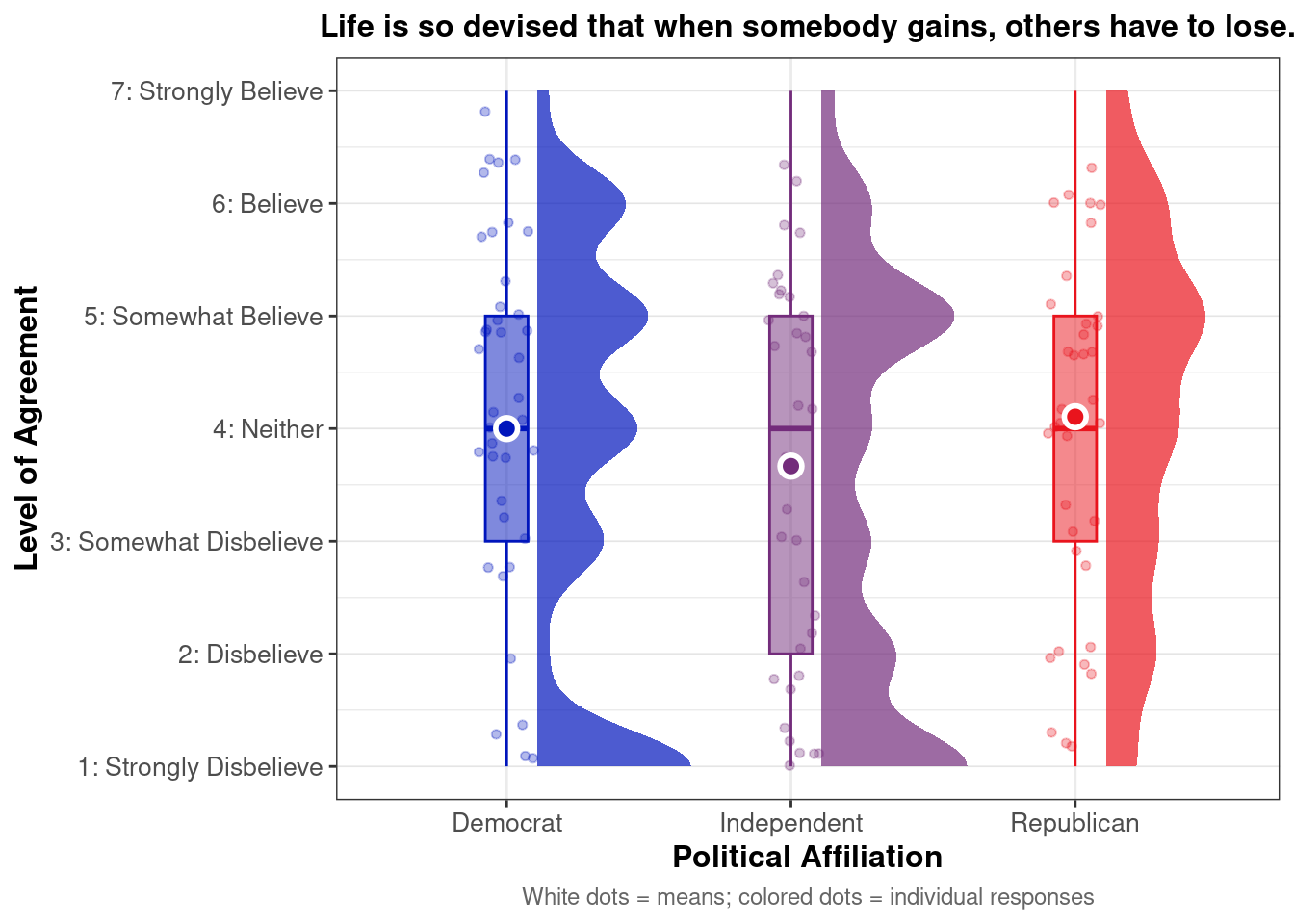
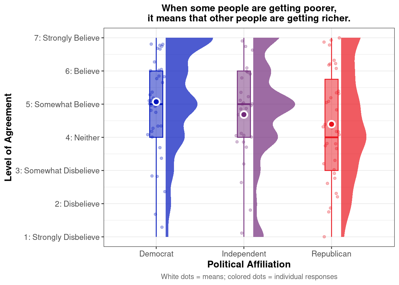
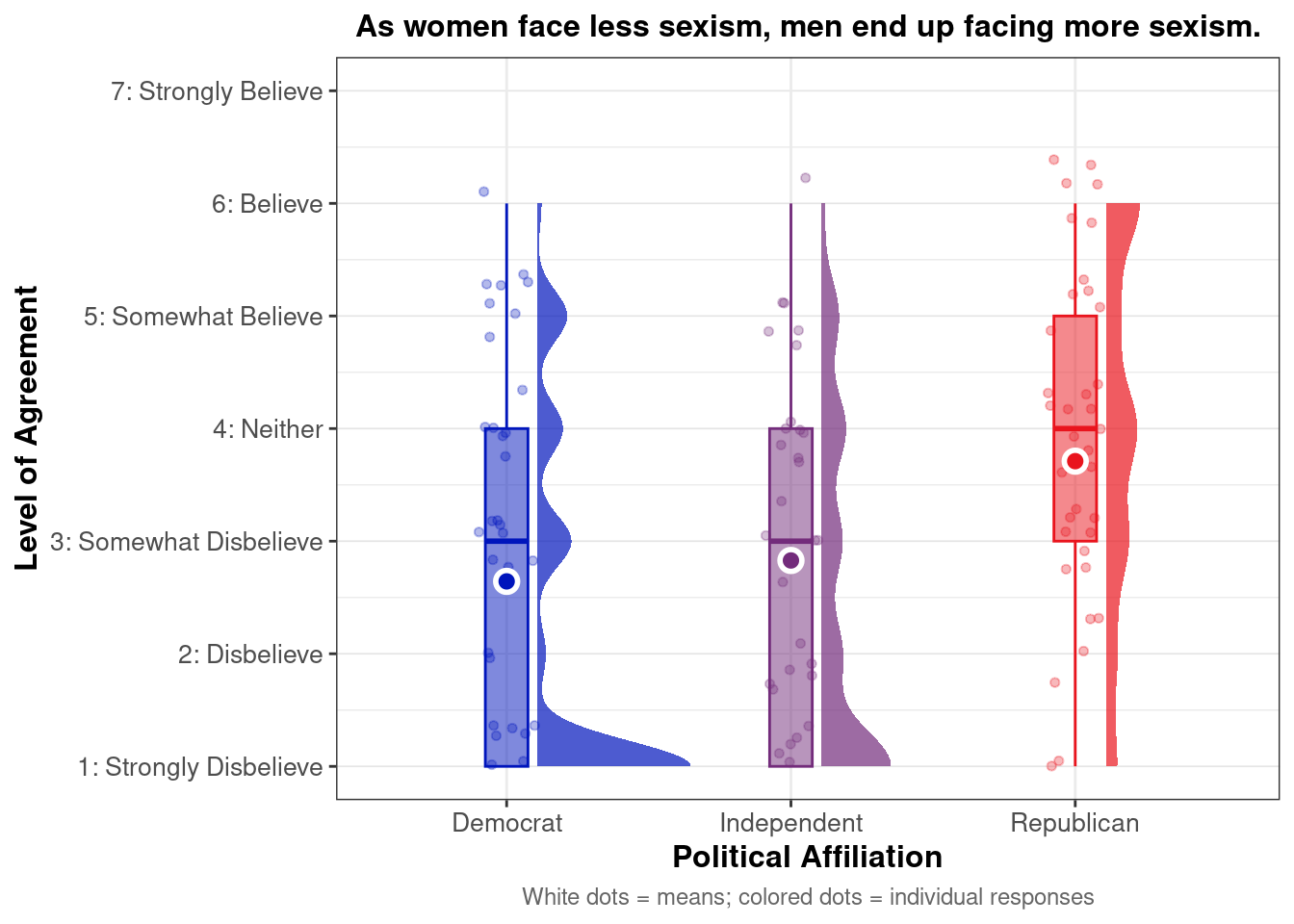
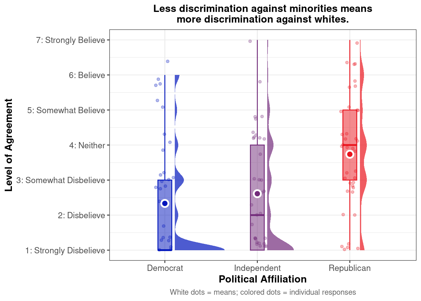
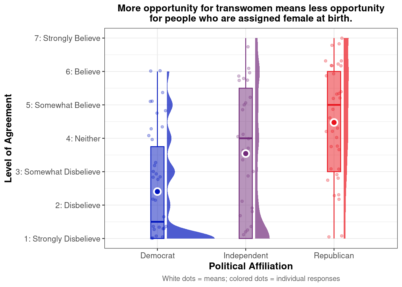
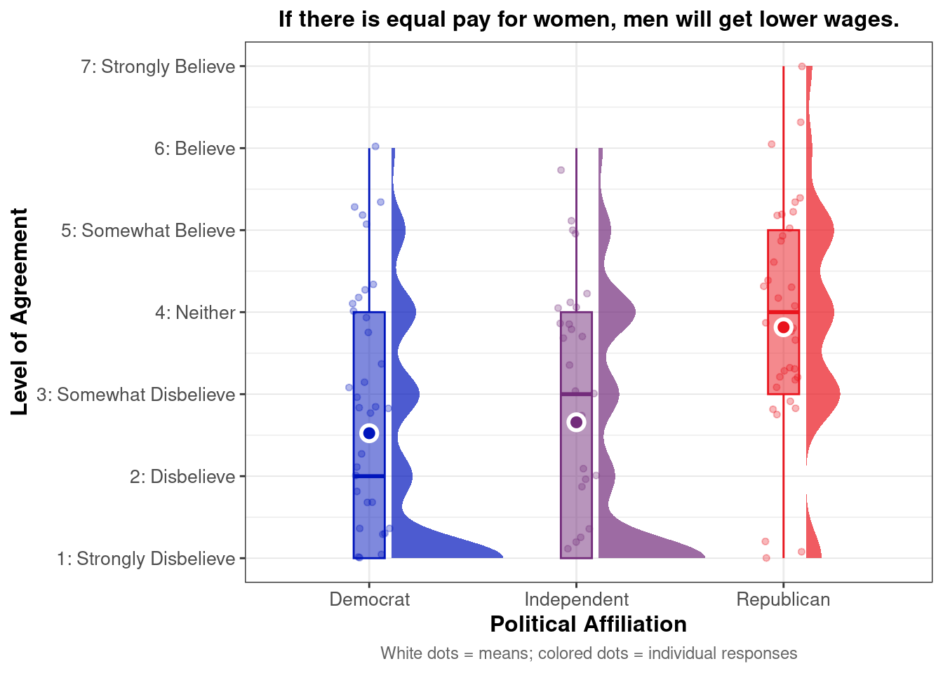
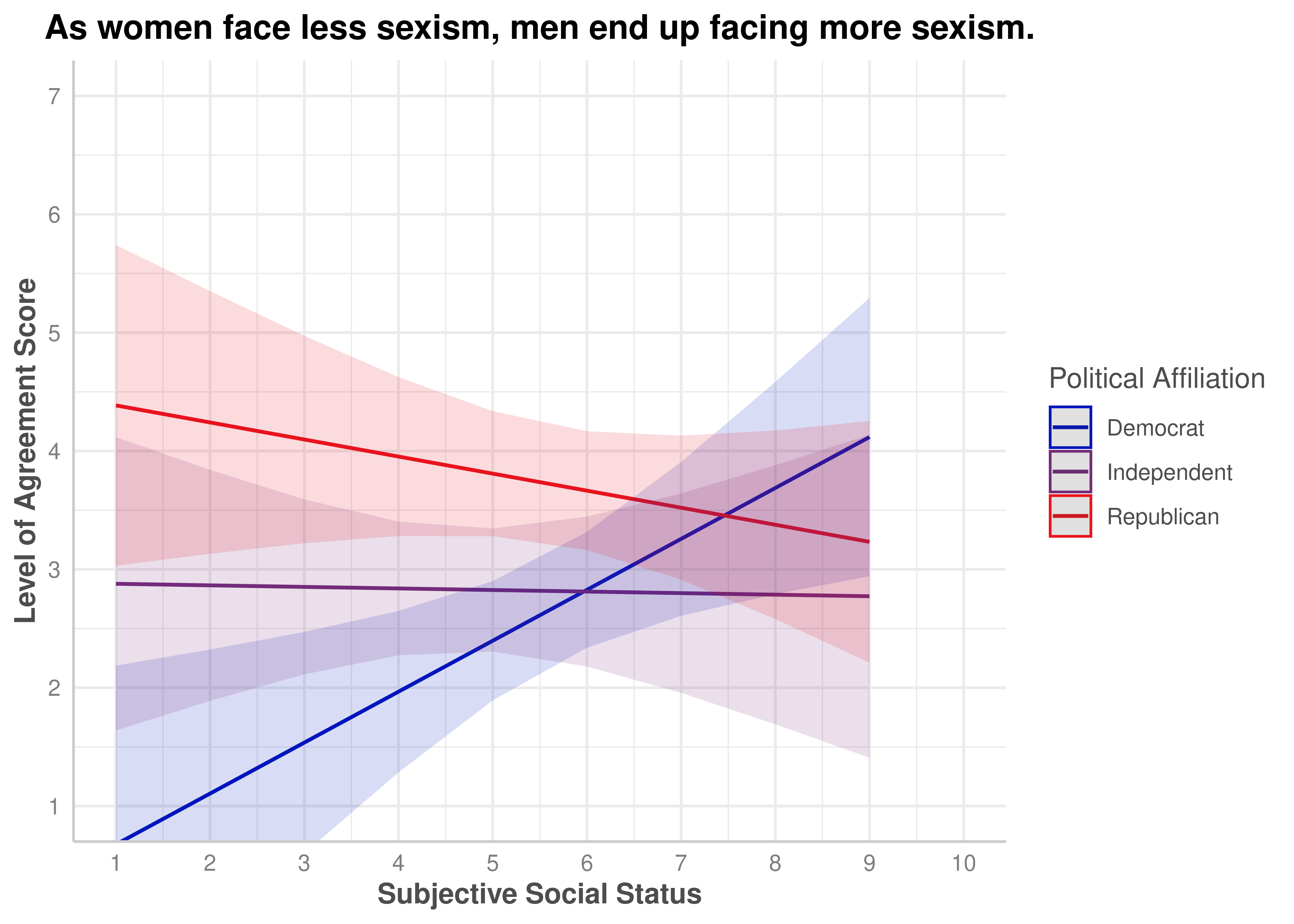
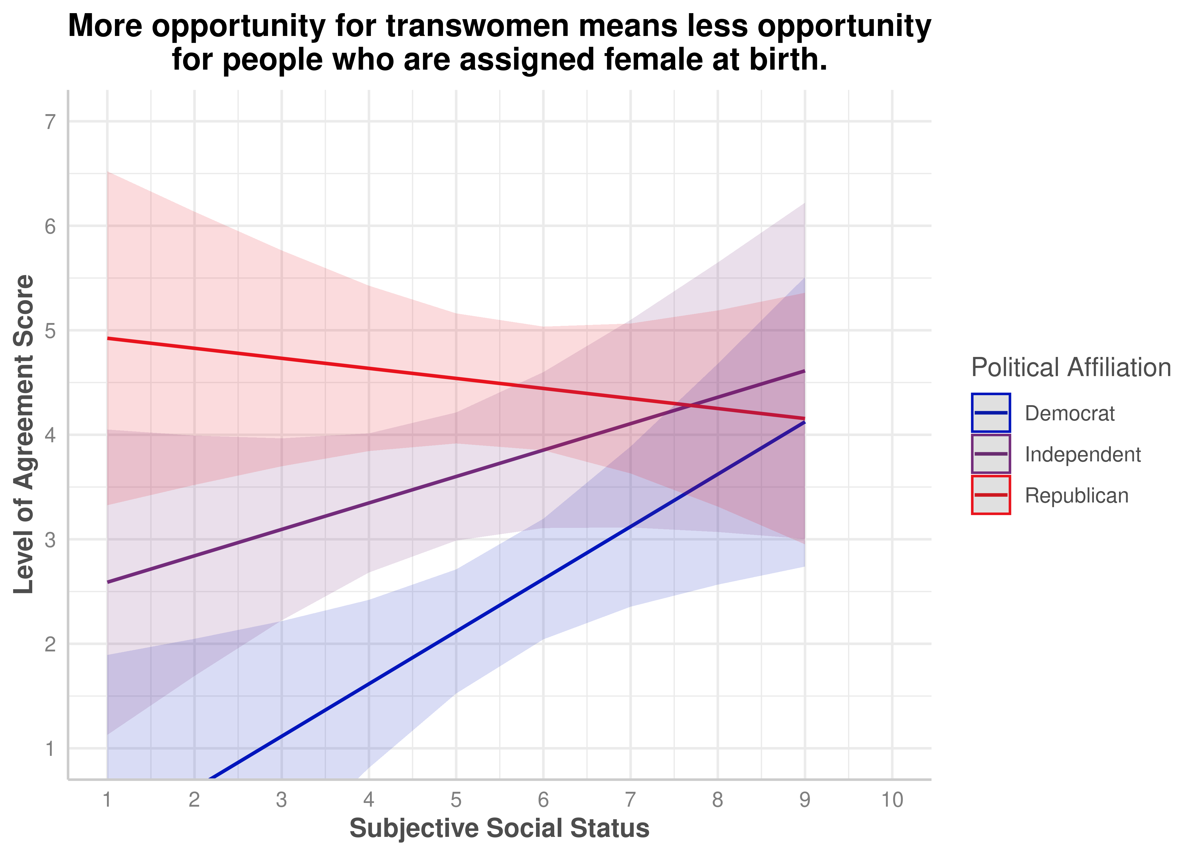
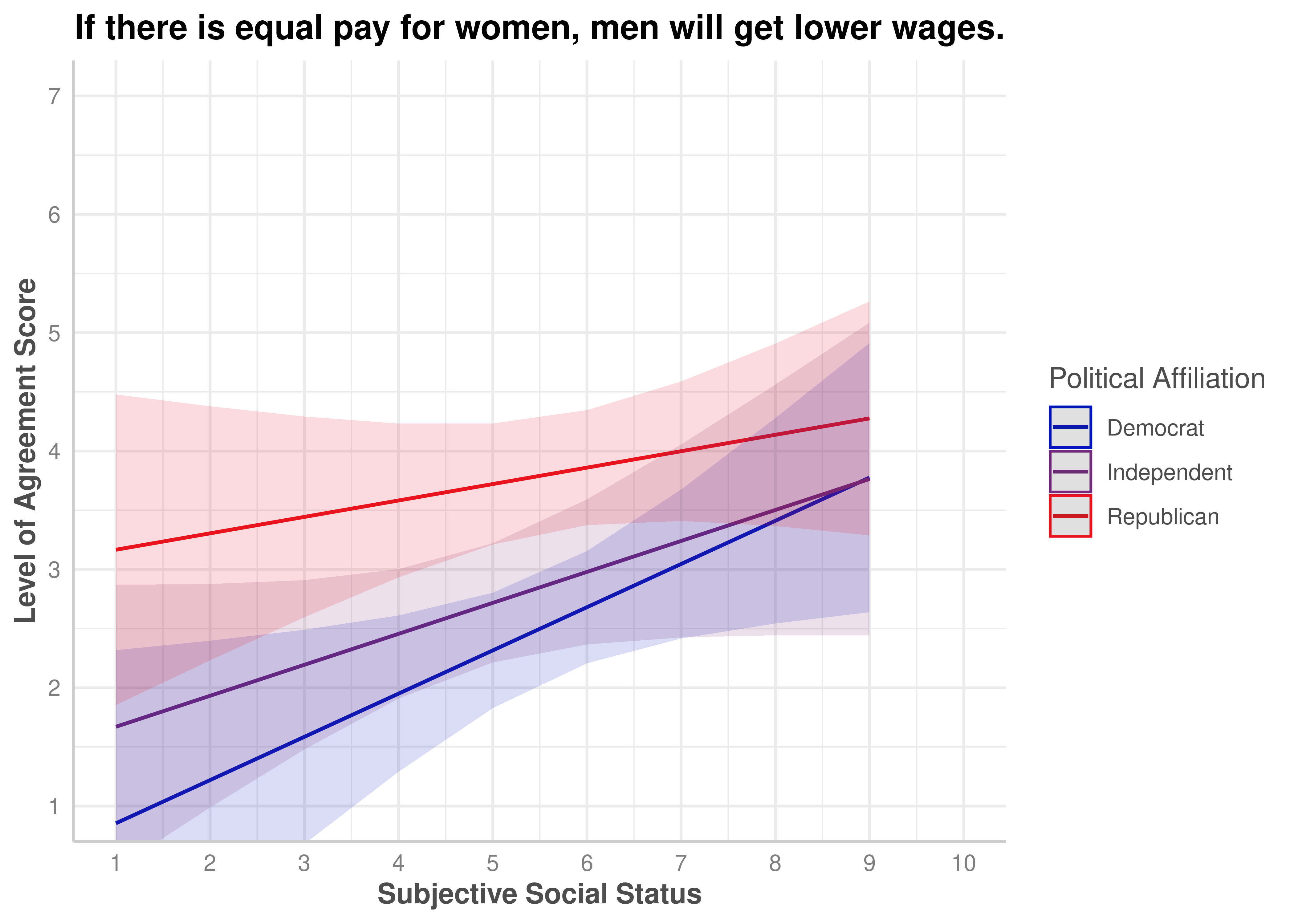
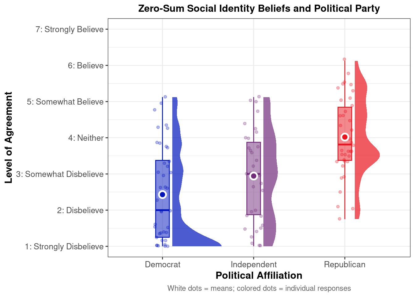
In contrast to decades of existing research demonstrating that social identities explain political party alignment, our findings suggest that a person’s beliefs about social identity groups—specifically zero-sum social identity beliefs—may matter more than a person’s social identity. A series of eleven ANCOVAs revealed that zero-sum beliefs differed systematically by political party affiliation across multiple domains, with Republicans reporting consistently higher endorsement of zero-sum social identity beliefs compared to Independents and Democrats. These intercept differences were largest for transgender opportunity beliefs (b = 5.409, p < .001) and gender-based sexism beliefs (b = 4.284, p < .001). For transgender opportunity beliefs, the intercept for Republicans was 5.41. This indicates that at the lowest level of subjective social status, Republicans scored 5.409 points higher than Democrats on the belief that “More opportunity for transwomen means less opportunity for people who are assigned female at birth,” almost reaching the upper limit of a 7-point scale. Similarly, for gender-based sexist beliefs, the intercept for Republicans was b = 4.284. This indicates that among the lowest-ranking groups, Republicans scored 4.284 points higher than Democrats on the belief that “As women face less sexism, men end up facing more sexism.” These findings suggest that zero-sum thinking represents the most pronounced political division in our sample within the domain of gender and identity.

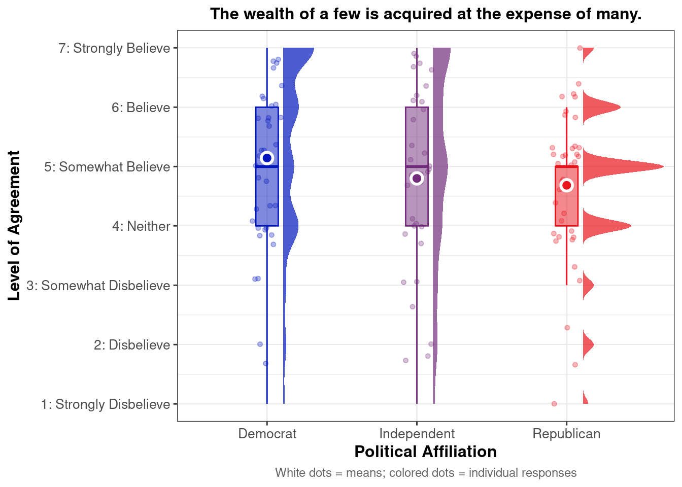
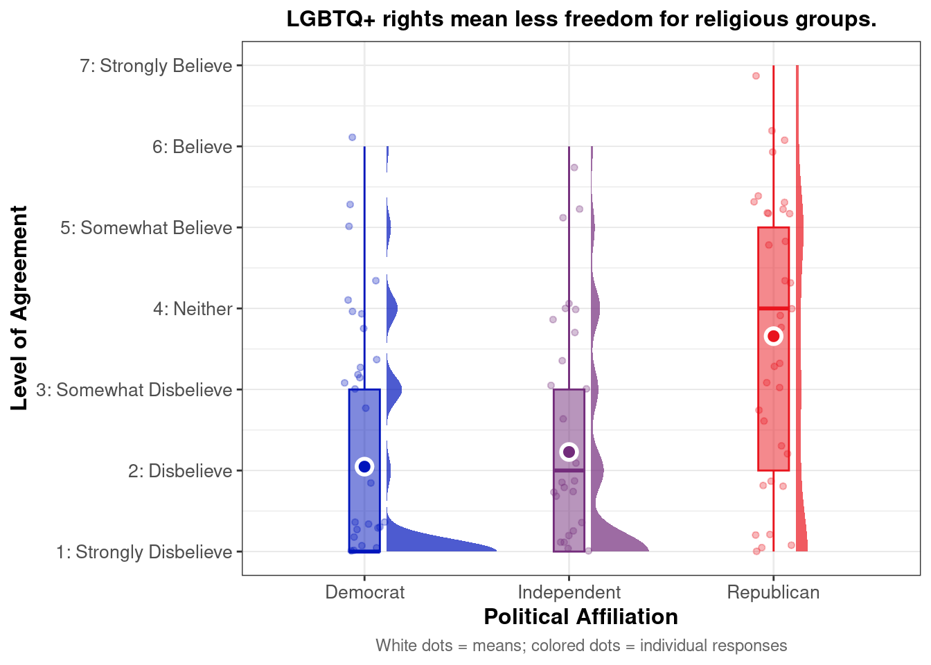
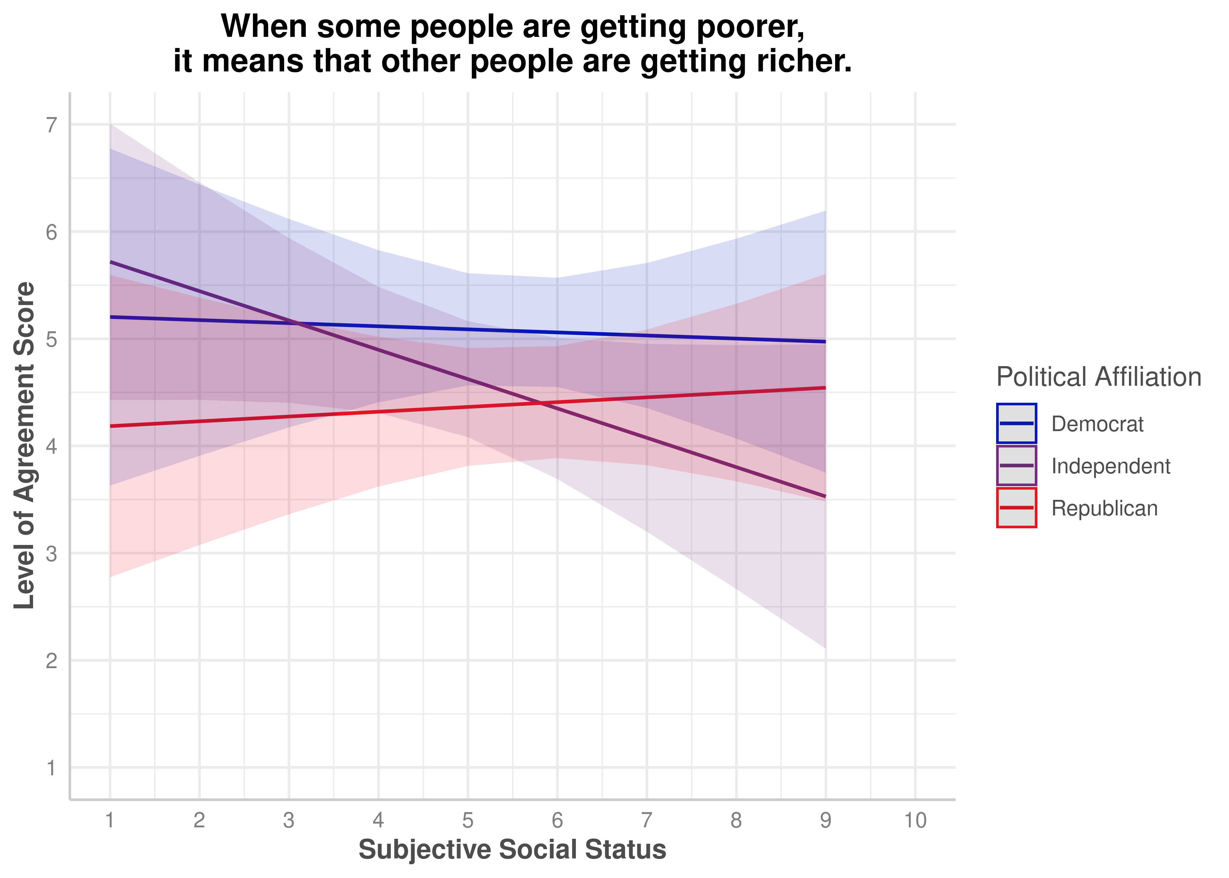
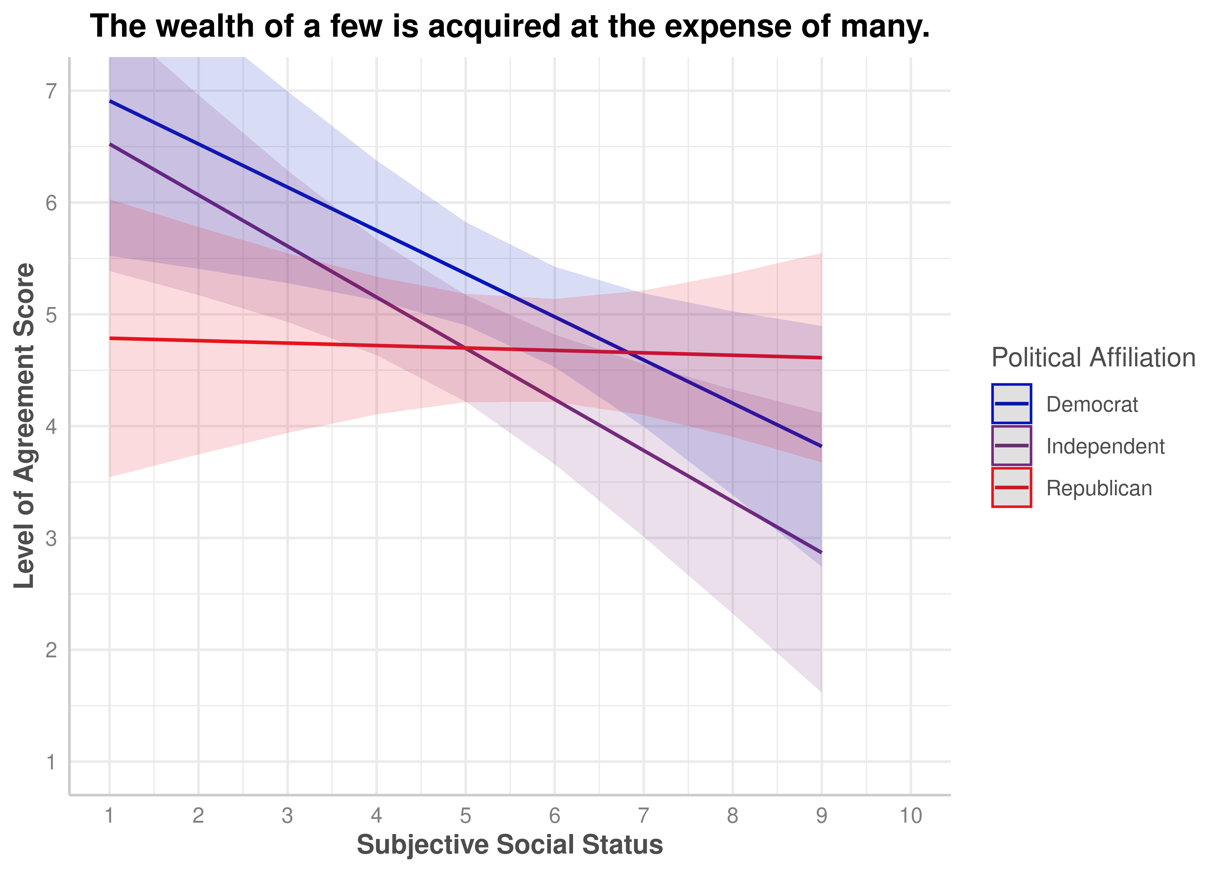
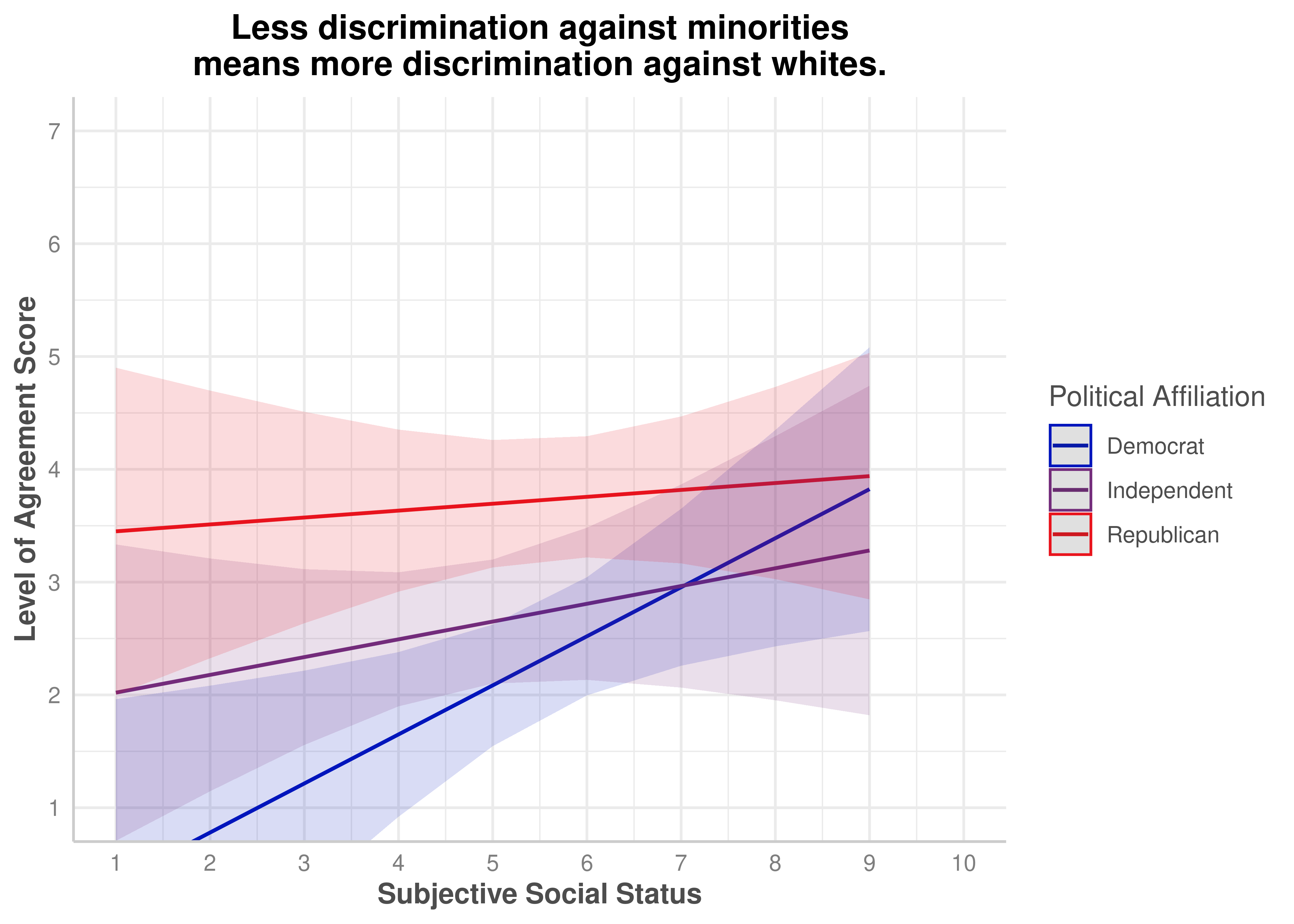
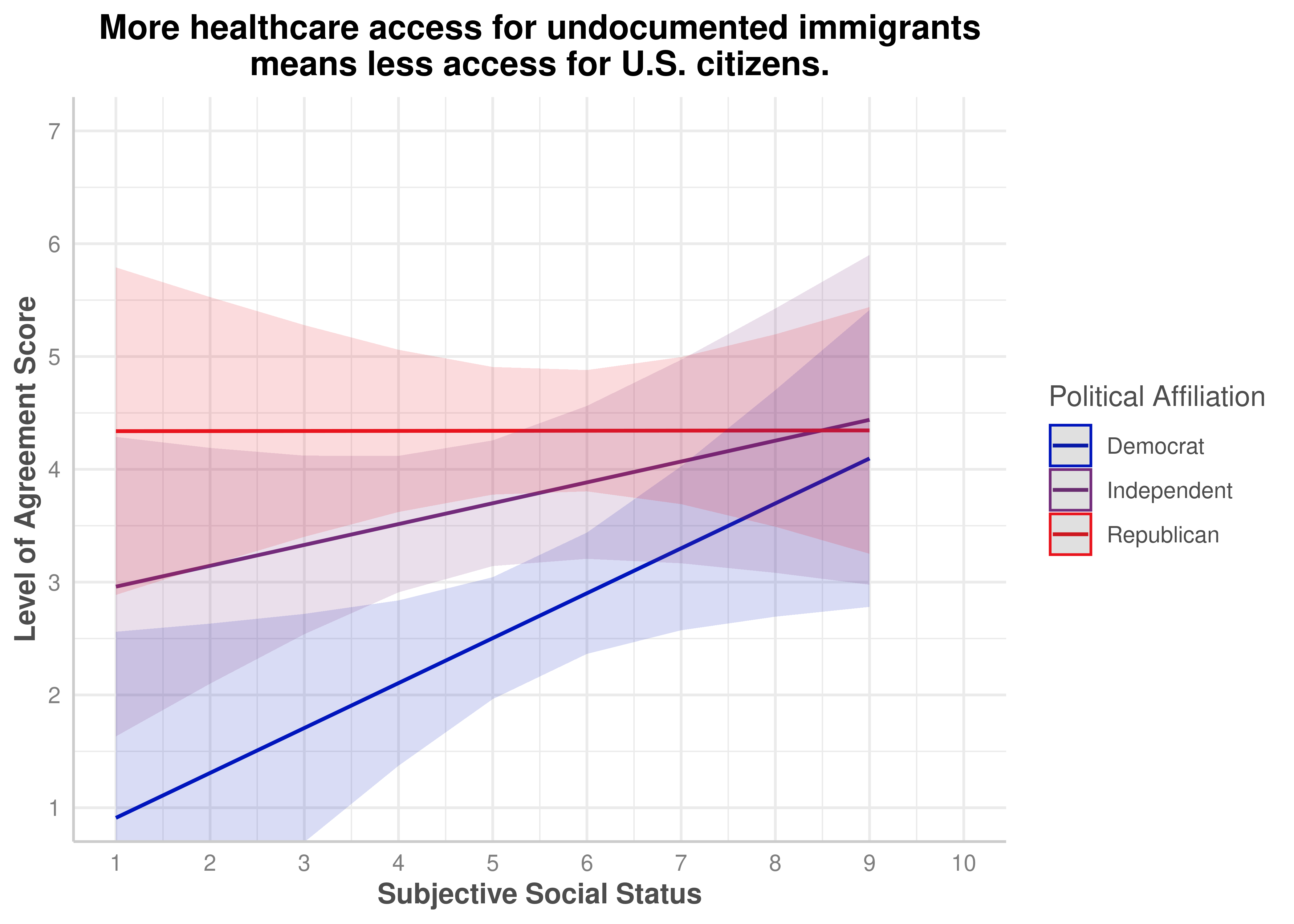
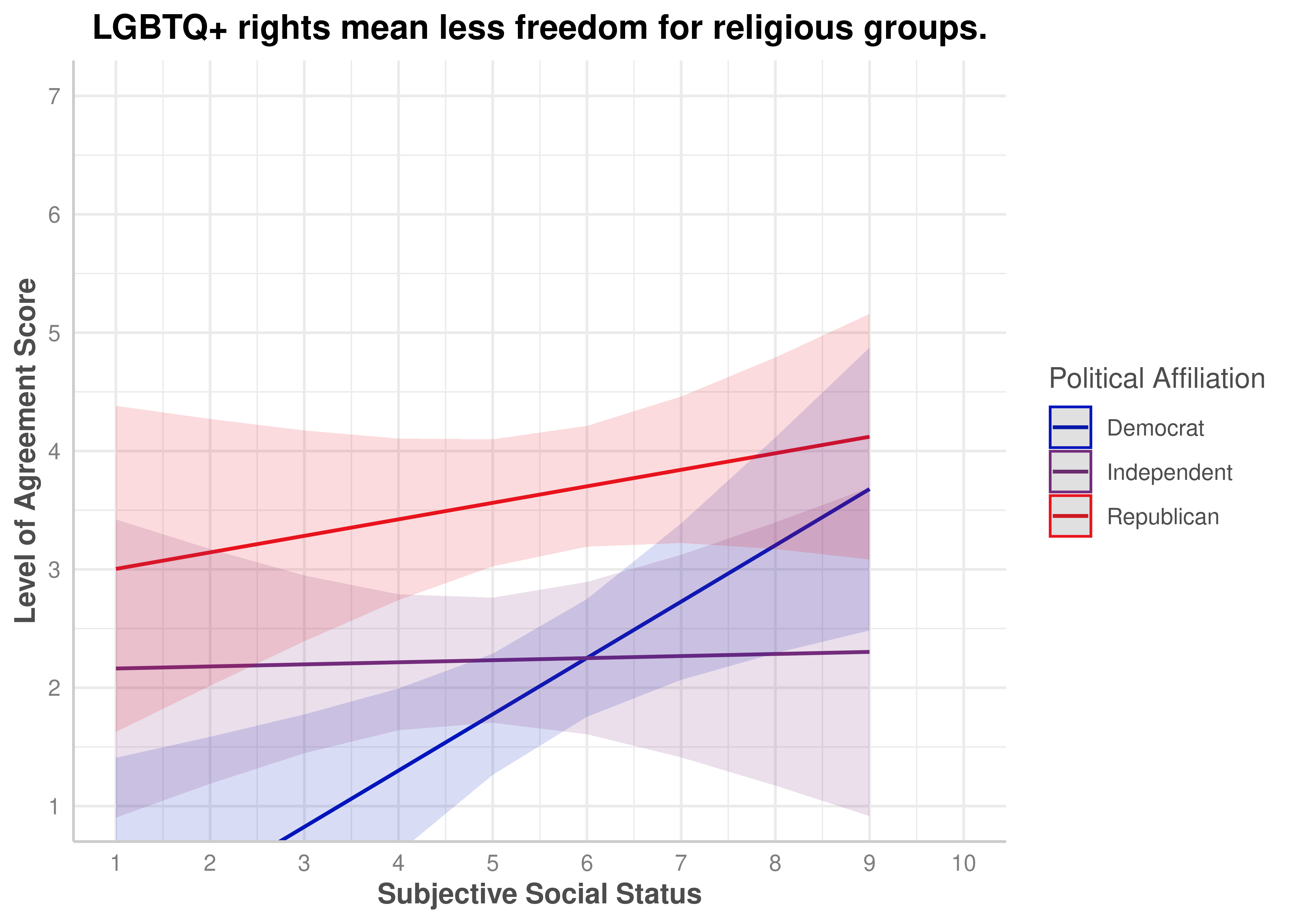
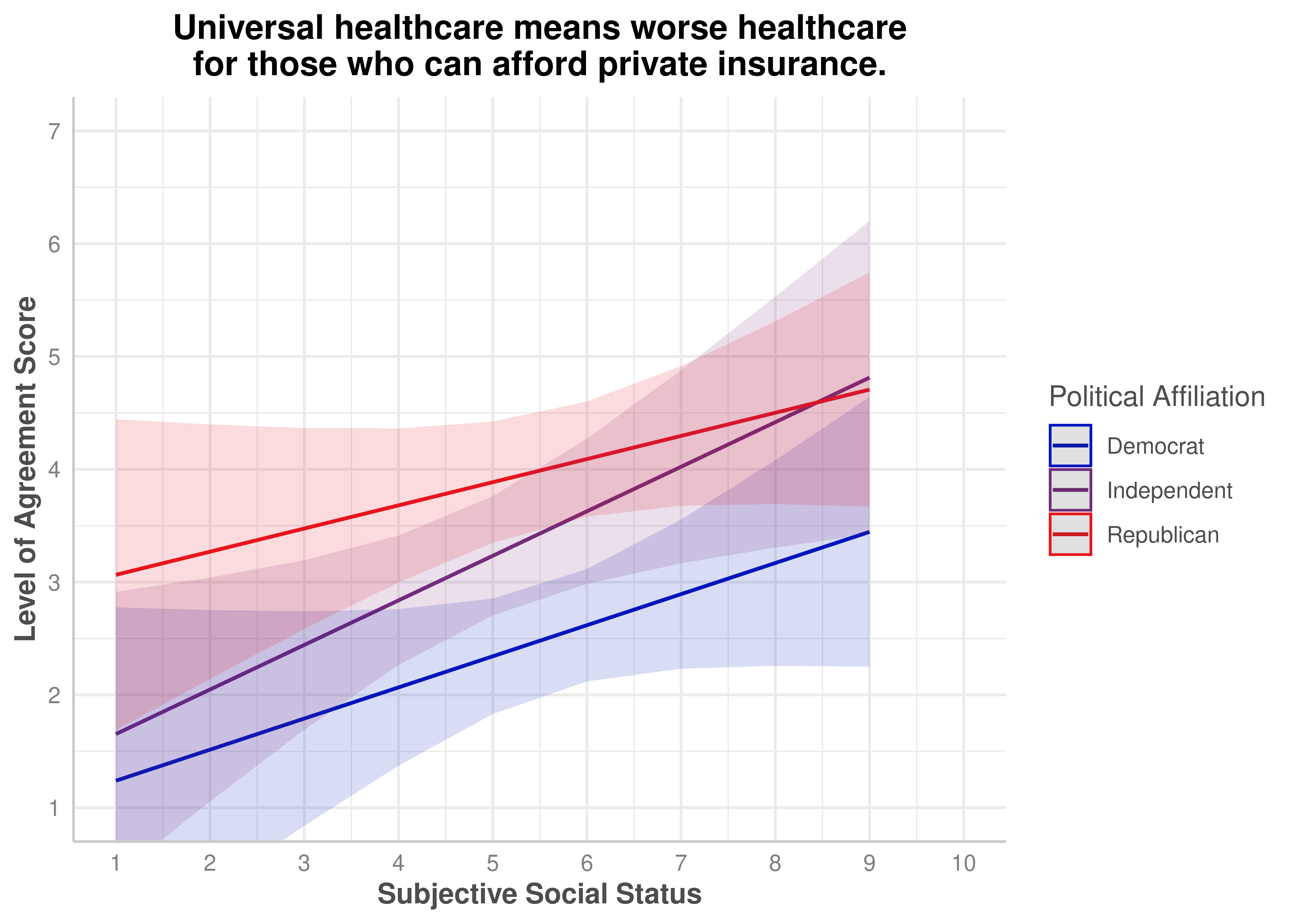
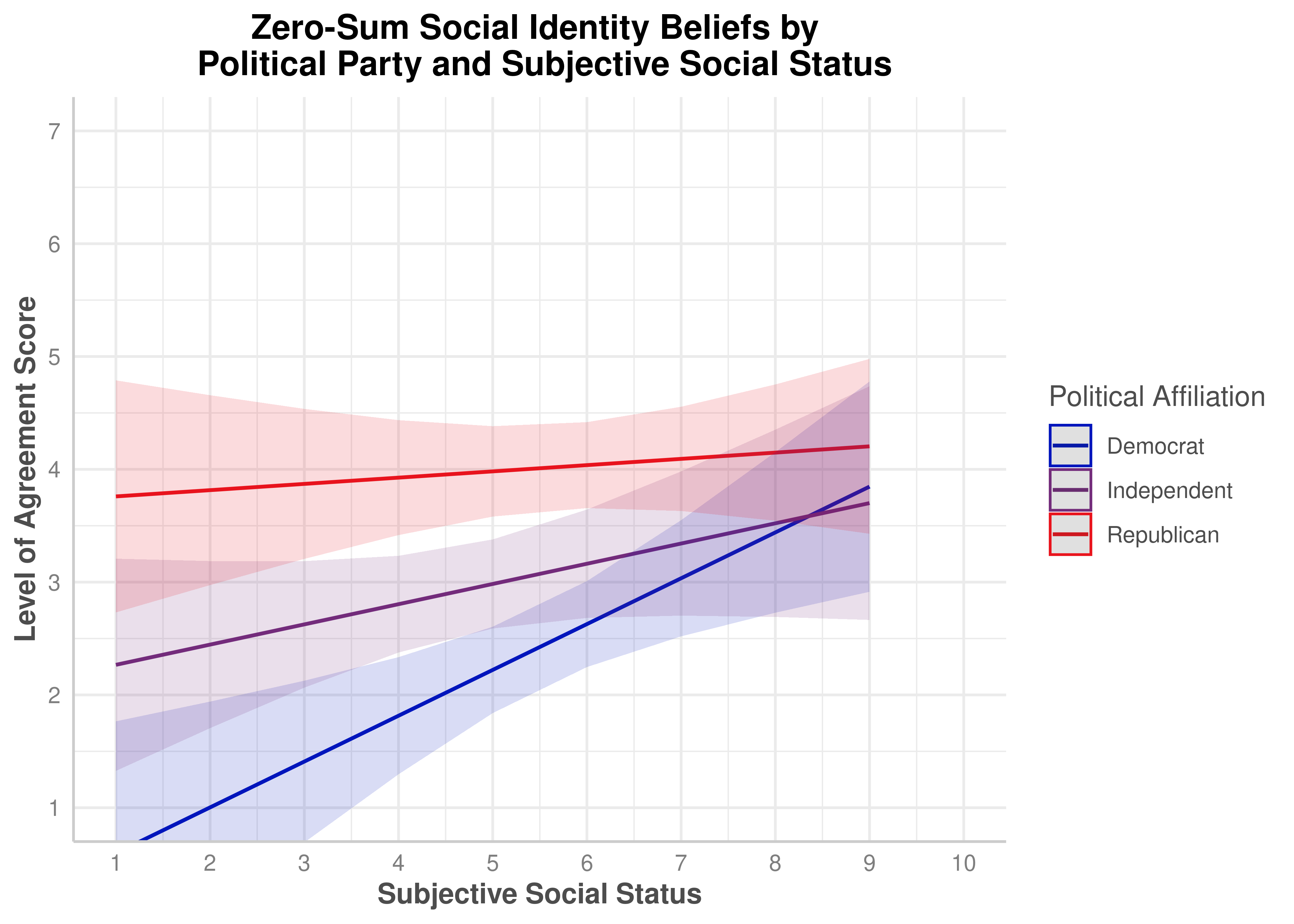
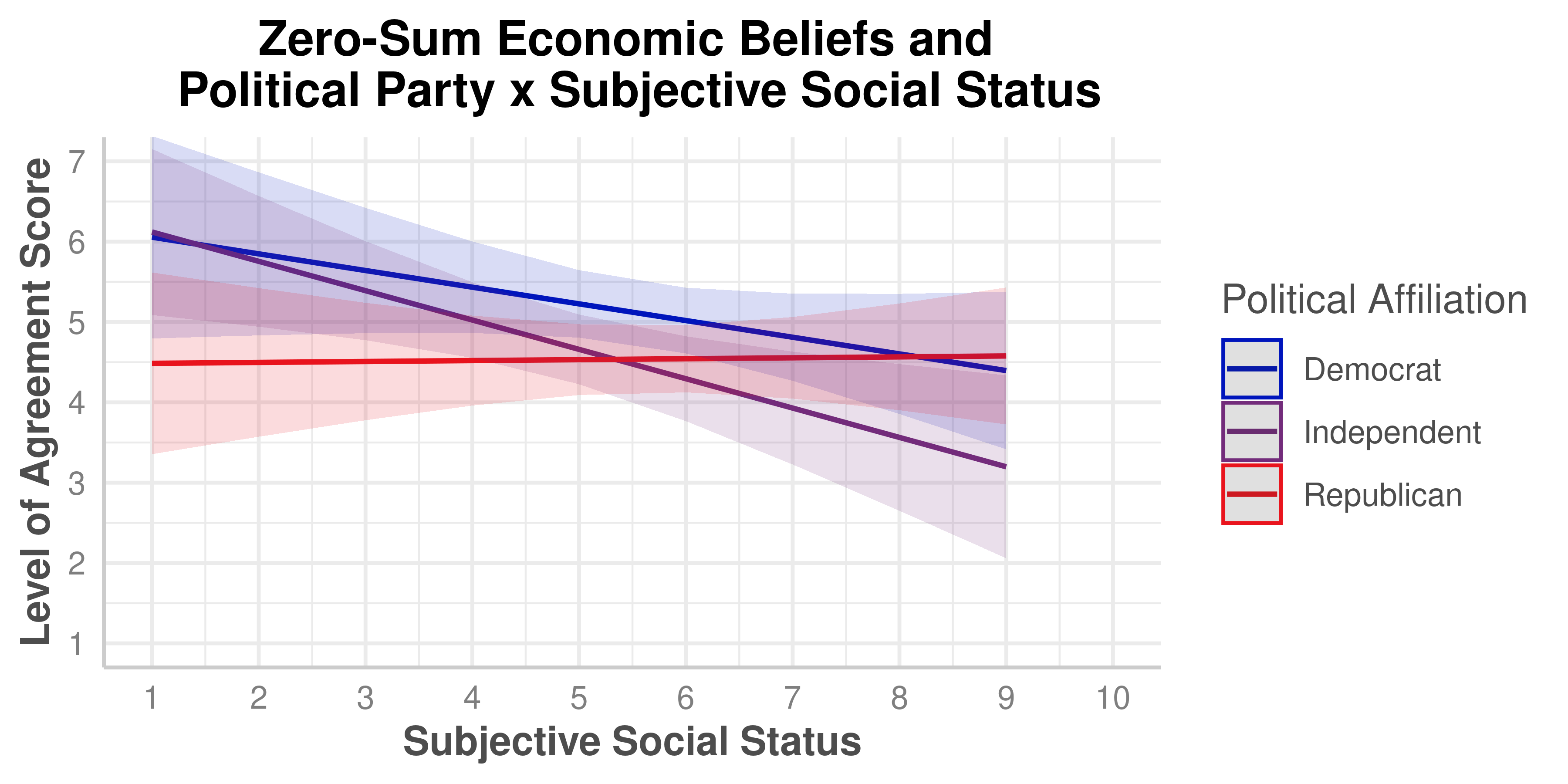
The current study also advances understanding of how subjective social status moderates zero-sum thinking differently across political groups. The study found significant subjective social status × party affiliation interactions in four areas: wealth inequality (F= 4.064, p = .002), gender-based sexism (F = 3.831, p = .003), transgender opportunities (F = 7.143, p < .001), and LGBTQ+ rights (F = 6.857, p < .001). Notably, in all four areas, higher subjective social status was associated with a higher level of identification with zero-sum thinking among Democrats. However, the positive correlation between perceived subjective social status and zero-sum thinking weakened or even reversed for Republicans and independents. For example, regarding gender-based sexist beliefs, the interaction between social status and Republicans was significant (b = −0.574, p = .007), while the interaction between social status and independents was significant (b = −0.444, p = .045). This difference suggests that perceived subjective social status may vary based on political identity, which requires further investigation. These findings indicate that zero-sum and social identity beliefs are one dimension of political polarization in contemporary America. These beliefs do not reflect simple partisan divisions but appear to be constructed from the intersection of political orientation and perceived social status. Future research should examine the causal relationship between perceived social status and zero-sum thinking within political groups and explore whether interventions targeting zero-sum and social identity beliefs can effectively reduce political polarization.

Andrews-Fearon, P., & Davidai, S. (2023). Is status a zero-sum game? Zero-sum beliefs increase people’s preference for dominance but not prestige. Journal of Experimental Psychology: General, 152(2), 389–409. https://doi.org/10.1037/xge0001282

Barber, M., & Pope, J. C. (2024). The Crucial Role of Race in Twenty-First Century US Political Realignment. Public Opinion Quarterly, 88(1), 149–160. https://doi.org/10.1093/poq/nfad063

Boland, F. K., & Davidai, S. (2024). Zero-sum beliefs and the avoidance of political conversations. Communications Psychology, 2(1), 43. https://doi.org/10.1038/s44271-024-00095-4

Brown, N. D., Jacoby-Senghor, D. S., & Raymundo, I. (2022). If you rise, I fall: Equality is prevented by the misperception that it harms advantaged groups. Science Advances, 8(18), eabm2385. https://doi.org/10.1126/sciadv.abm2385

Chinoy, S., Nunn, N., Sequeira, S., & Stantcheva, S. (2023). Zero-sum Thinking and the Roots of US Political Differences (w31688; p. w31688). National Bureau of Economic Research. https://doi.org/10.3386/w31688

Davidai, S., & Ongis, M. (2019). The politics of zero-sum thinking: The relationship between political ideology and the belief that life is a zero-sum game. Science Advances, 5(12), eaay3761. https://doi.org/10.1126/sciadv.aay3761

Davis, S., & Sequeira, S. (2024). Zero-Sum Thinking: Roots And Policy Implications. Hoover Institution. https://www.hoover.org/research/zero-sum-thinking-roots-and-policy-implications

Esses, V. M., Dovidio, J. F., Jackson, L. M., & Armstrong, T. L. (2001). The Immigration Dilemma: The Role of Perceived Group Competition, Ethnic Prejudice, and National Identity. Journal of Social Issues, 57(3), 389–412. https://doi.org/10.1111/0022-4537.00220

Hornborg, A. (2003). Cornucopia or Zero-Sum Game? The Epistemology of Sustainability. Journal of World-Systems Research, 205–216. https://doi.org/10.5195/jwsr.2003.245

Meyer, N. (2025). The Democrats Embrace Dealignment. Catalyst, 8(4), 8–51.

Nadeem, R. (2024, April 9). Changing Partisan Coalitions in a Politically Divided Nation. Pew Research Center. https://www.pewresearch.org/politics/2024/04/09/changing-partisan-coalitions-in-a-politically-divided-nation/

Norton, M. I., & Sommers, S. R. (2011). Whites See Racism as a Zero-Sum Game That They Are Now Losing. Perspectives on Psychological Science, 6(3), 215–218. https://doi.org/10.1177/1745691611406922

Rasmussen, R., Levari, D. E., Akhtar, M., Crittle, C. S., Gately, M., Pagan, J., Brennen, A., Cashman, D., Wulff, A. N., Norton, M. I., Sommers, S. R., & Urry, H. L. (2022). White (but Not Black) Americans Continue to See Racism as a Zero-Sum Game; White Conservatives (but Not Moderates or Liberals) See Themselves as Losing. Perspectives on Psychological Science, 17(6), 1800–1810. https://doi.org/10.1177/17456916221082111

Różycka-Tran, J., Boski, P., & Wojciszke, B. (2015). Belief in a Zero-Sum Game as a Social Axiom: A 37-Nation Study. Journal of Cross-Cultural Psychology, 46(4), 525–548. https://doi.org/10.1177/0022022115572226

Wickham, H., Çetinkaya-Rundel, M., & Grolemund, G. (2016). Whole game – R for Data Science (2e). https://r4ds.hadley.nz/whole-game.html

Wilkins, C. L., Wellman, J. D., Babbitt, L. G., Toosi, N. R., & Schad, K. D. (2015). You can win but I can’t lose: Bias against high-status groups increases their zero-sum beliefs about discrimination. Journal of Experimental Social Psychology, 57, 1–14. https://doi.org/10.1016/j.jesp.2014.10.008

Wojciszke, B., Baryła, W., & Różycka, J. (2009). Wiara w życie jako grę o sumie zerowej [Zero-Sum Game Belief]. In Między przeszłością a przyszłością. Szkice z psychologii politycznej [Between the past and the future. Essays from political psychology] (pp. 179–188). Warsaw: Polish Academy of Sciences Press.

Wong, Y. J., Klann, E. M., Bijelić, N., & Aguayo, F. (2017). The link between men’s zero-sum gender beliefs and mental health: Findings from Chile and Croatia. Psychology of Men & Masculinity, 18(1), 12–19. https://doi.org/10.1037/men0000035