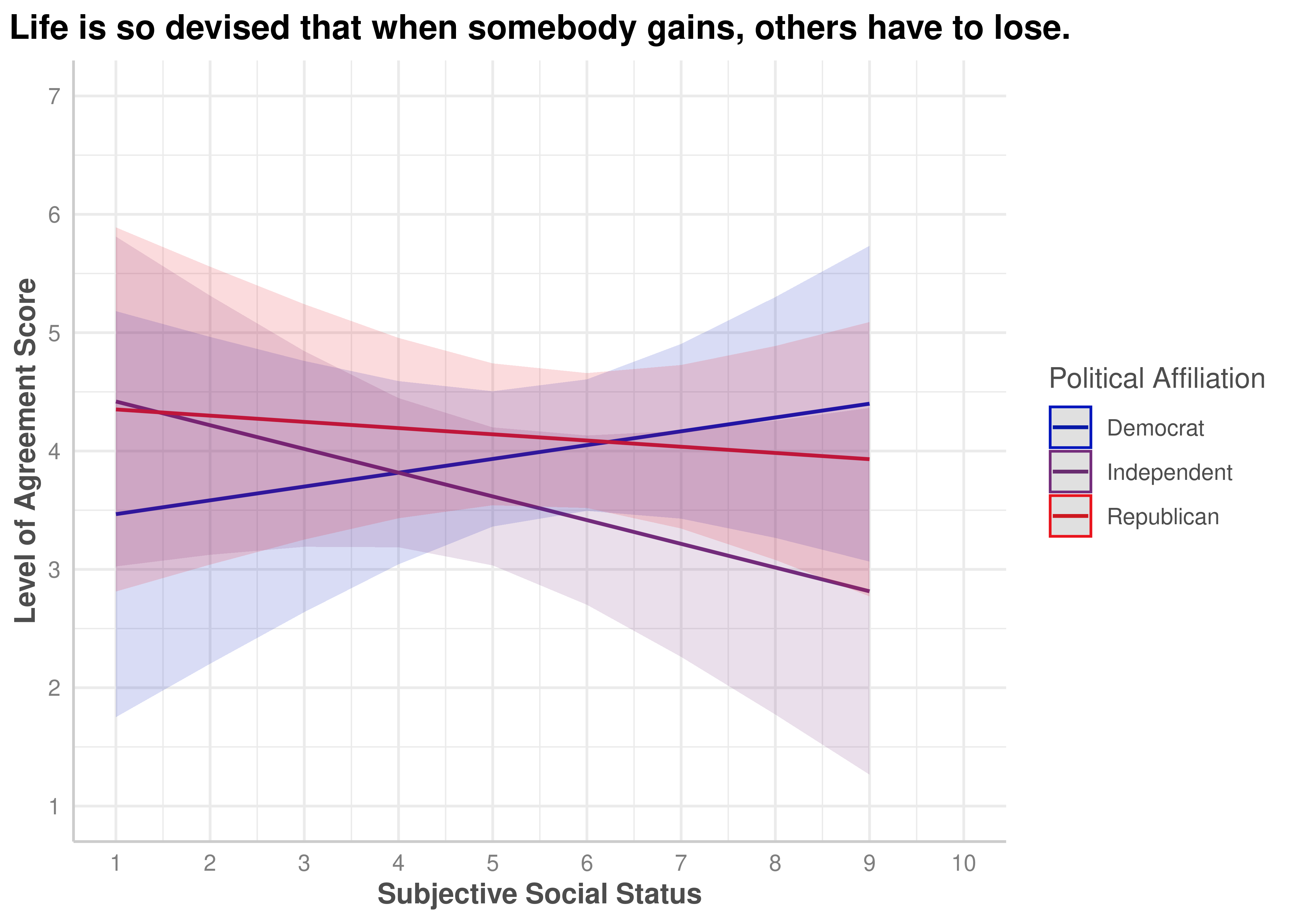
(ZEROSUM_1) Life is so devised that when somebody gains, others have to lose.
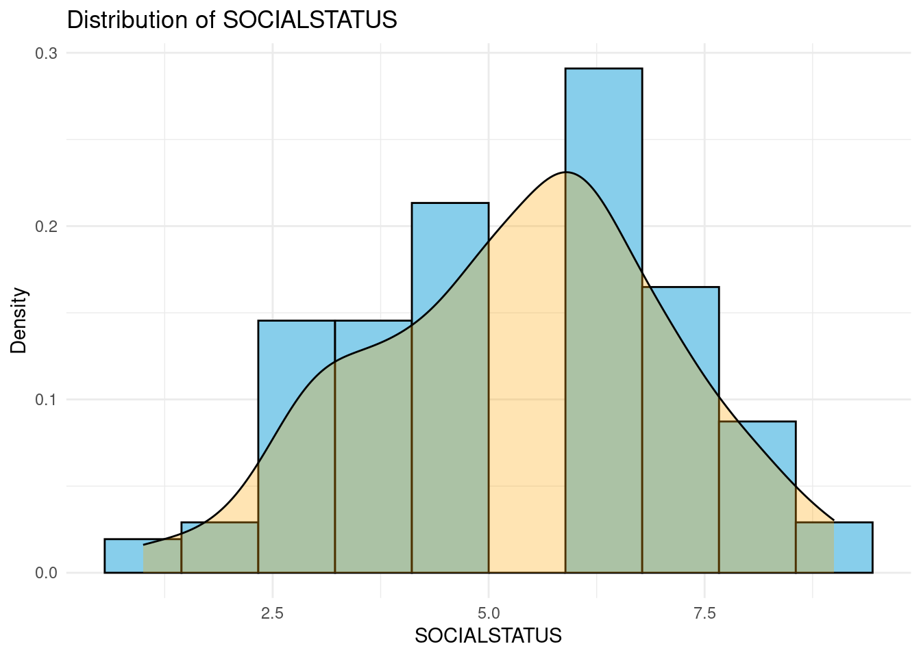
SOCIALSTATUS
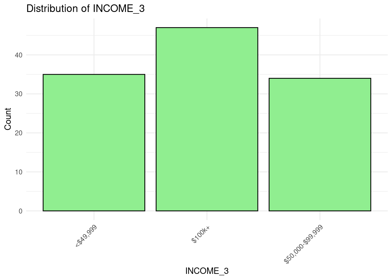
INCOME
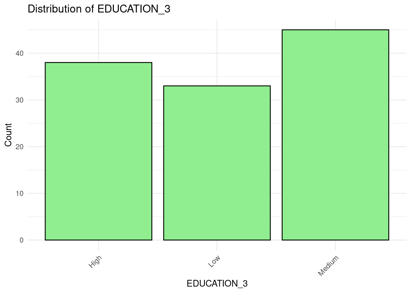
EDUCATION
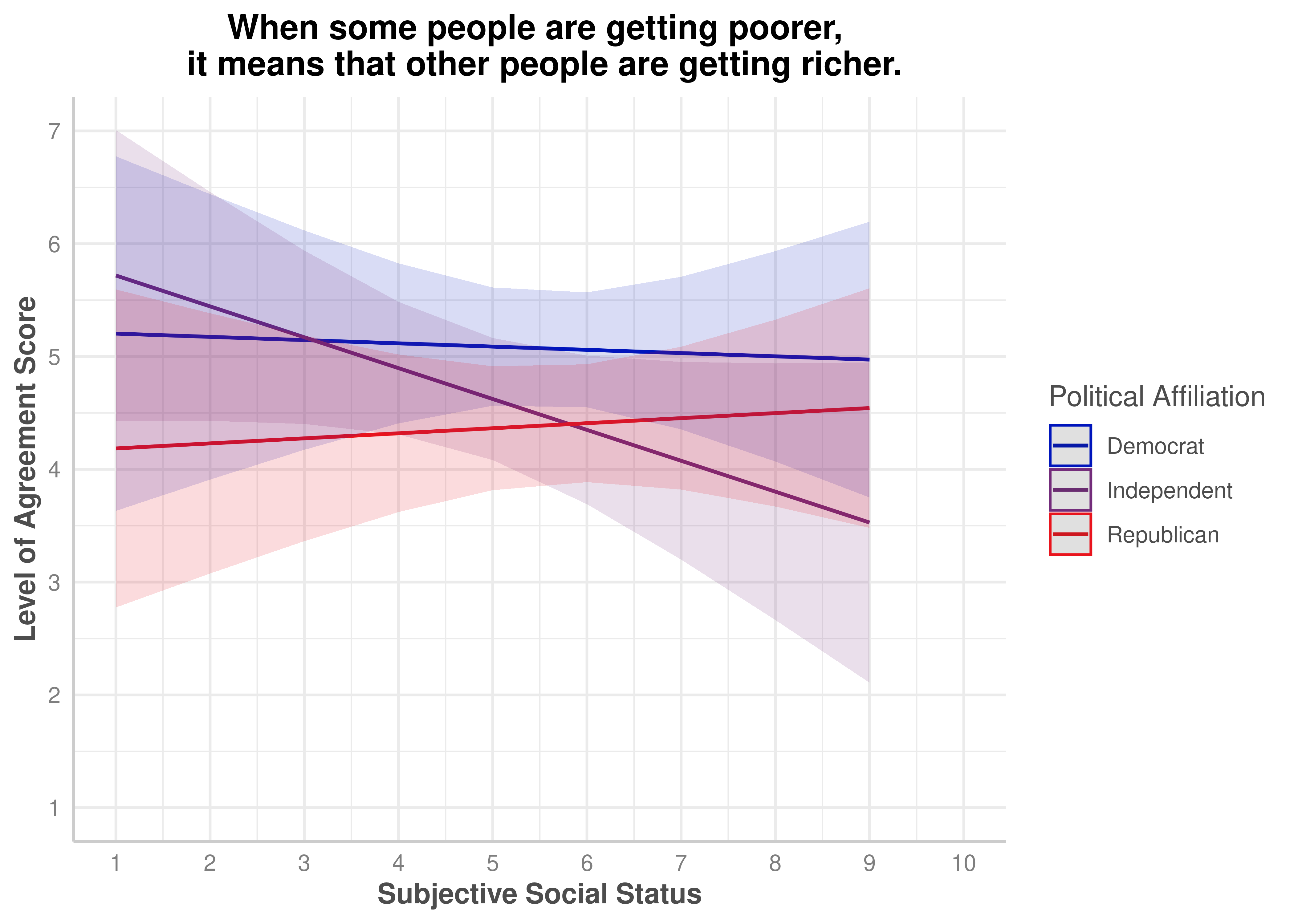
(ZEROSUM_2) When some people are getting poorer, it means that other people are getting richer.
SOCIALSTATUS
INCOME
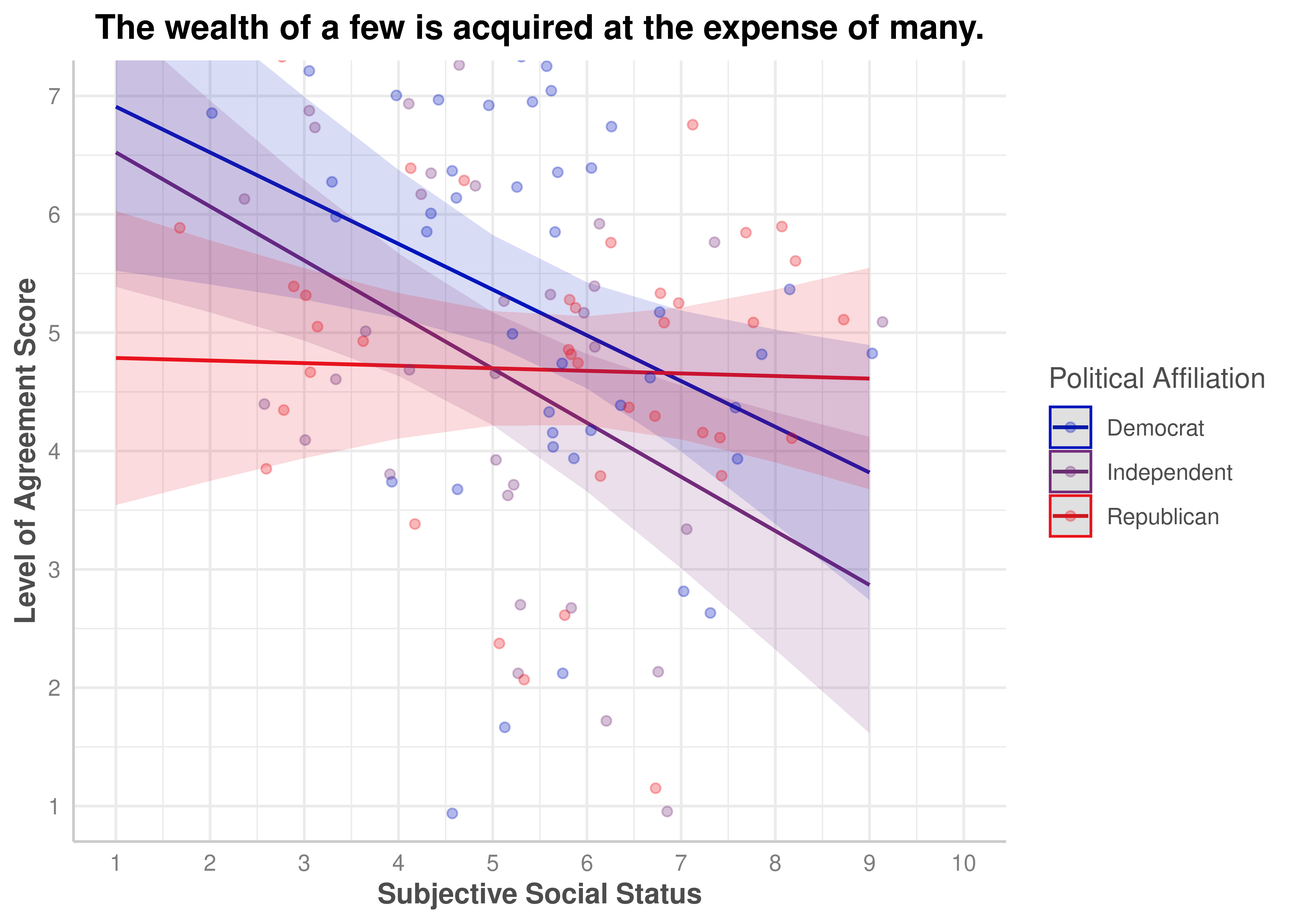
(ZEROSUM_3) The wealth of a few is acquired at the expense of many.
SOCIALSTATUS
INCOME
(ZEROSUM_4) As women face less sexism, men end up facing more sexism.
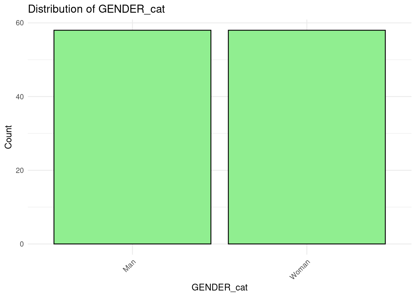
GENDER_cat
(ZEROSUM_5) Less discrimination against minorities means more discrimination against whites.
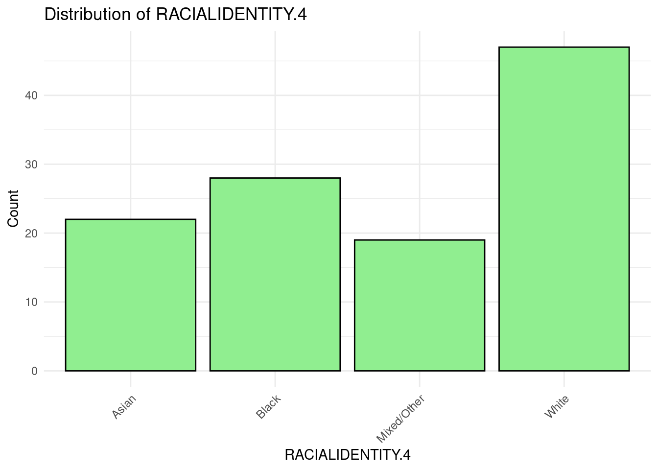
RACIALIDENTITY.4
SOCIALSTATUS
(ZEROSUM_6) More opportunity for transwomen means less opportunity for people assigned female at birth.
GENDER_cat
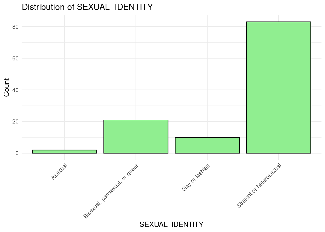
SEXUAL_IDENTITY
(ZEROSUM_7) More healthcare access for undocumented immigrants means less access for U.S. citizens.
No direct social identity measured in dataset
(ZEROSUM_8) If there is equal pay for women, men will get lower wages.
GENDER_cat
SOCIALSTATUS
(ZEROSUM_9) LGBTQ+ rights mean less freedom for religious groups.
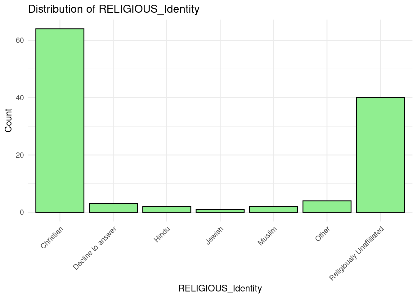
RELIGIOUS_Identity
SEXUAL_IDENTITY
(ZEROSUM_10) Accessible healthcare for people with disabilities means longer wait times for others.
No disability variable in dataset
SOCIALSTATUS
(ZEROSUM_11) Universal healthcare means worse healthcare for those who can afford private insurance.
SOCIALSTATUS
INCOME
Analysis Plan
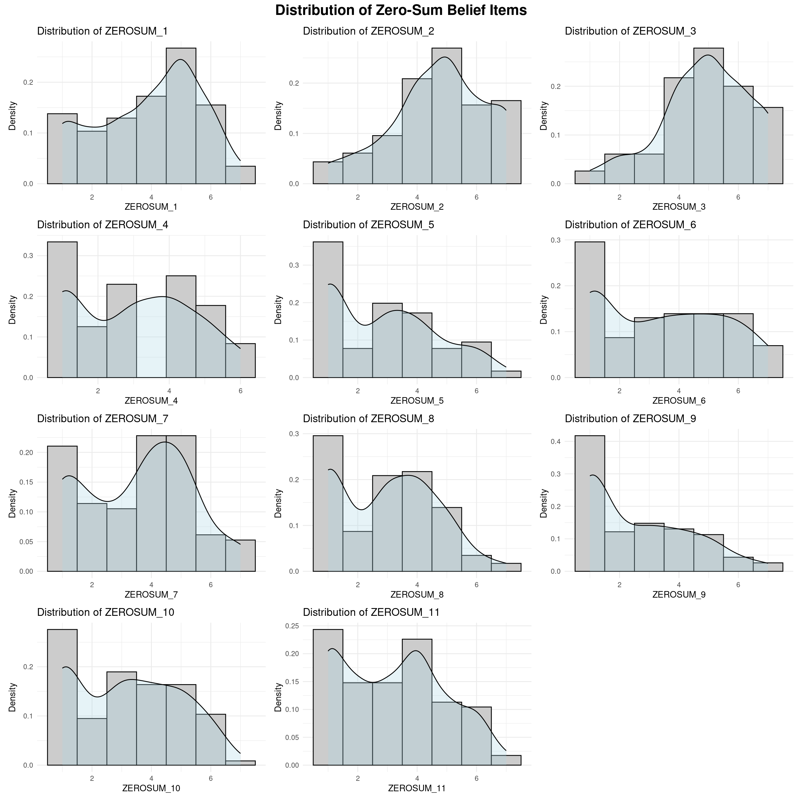
A total of 11 zero-sum belief items (ZEROSUM_1:ZEROSUM_11) covering economic, gender, racial, healthcare, and LGBTQ+ domains were analyzed. Analyses were conducted in R using series of two-way analysis of covariance (ANCOVA) models. Each model evaluated one zero-sum belief item as the outcome variable with subjective social status (SSS) as a continuous predictor and political party (Democrat, Republican, Independent) as a categorical predictor, along with their interaction term: \[\text{ZEROSUM}_i ~ \text{SOCIALSTATUS} \times \text{POLITICALPARTY}\] {#eq-ANCOVA analysis equation}
ANCOVA was selected over ANOVA for the SOCIALSTATUS predictor because SSS is measured on a continuous scale. Treating SSS as continuous in a regression framework allows estimation of whether the linear relationship between SSS and zero-sum beliefs differs across political party groups. POLITICALPARTY was coded as a categorical factor with Democrat as the reference group, allowing for direct comparisons between Republicans and Independents relative to Democrats.
Models were estimated in R using lm(). The F-statistic and model R-squared for each ANCOVA are reported to characterize overall model fit. Individual regression coefficients, standard errors, t-values, and p-values are inspected to characterize specific main effects and interactions.
We used the ggeffects package to predicted marginal means plots to visualize and interpret significant interaction patterns.
Additional Social Identity Variables
The manuscript also documents ANOVA analyses with categorical social identity variables for specific items (INCOME_3, GENDER_cat, RACIALIDENTITY.4, SEXUAL_IDENTITY_binary). These are addressed as complementary analyses and are not the primary focus of this plan. The core ANCOVA series centers on SOCIALSTATUS × POLITICALPARTY.
Result
Item
Zero-sum belief statement
Significant. interaction?
R²
ZEROSUM_1
Life is so devised that when somebody gains, others have to lose.
No
-.016
ZEROSUM_2
When some people are getting poorer, it means that other people are getting richer.
No
.015
ZEROSUM_3
The wealth of a few is acquired at the expense of many.
Yes, p = .002
.012
ZEROSUM_4
As women face less sexism, men end up facing more sexism.
Yes, p = .003
.111
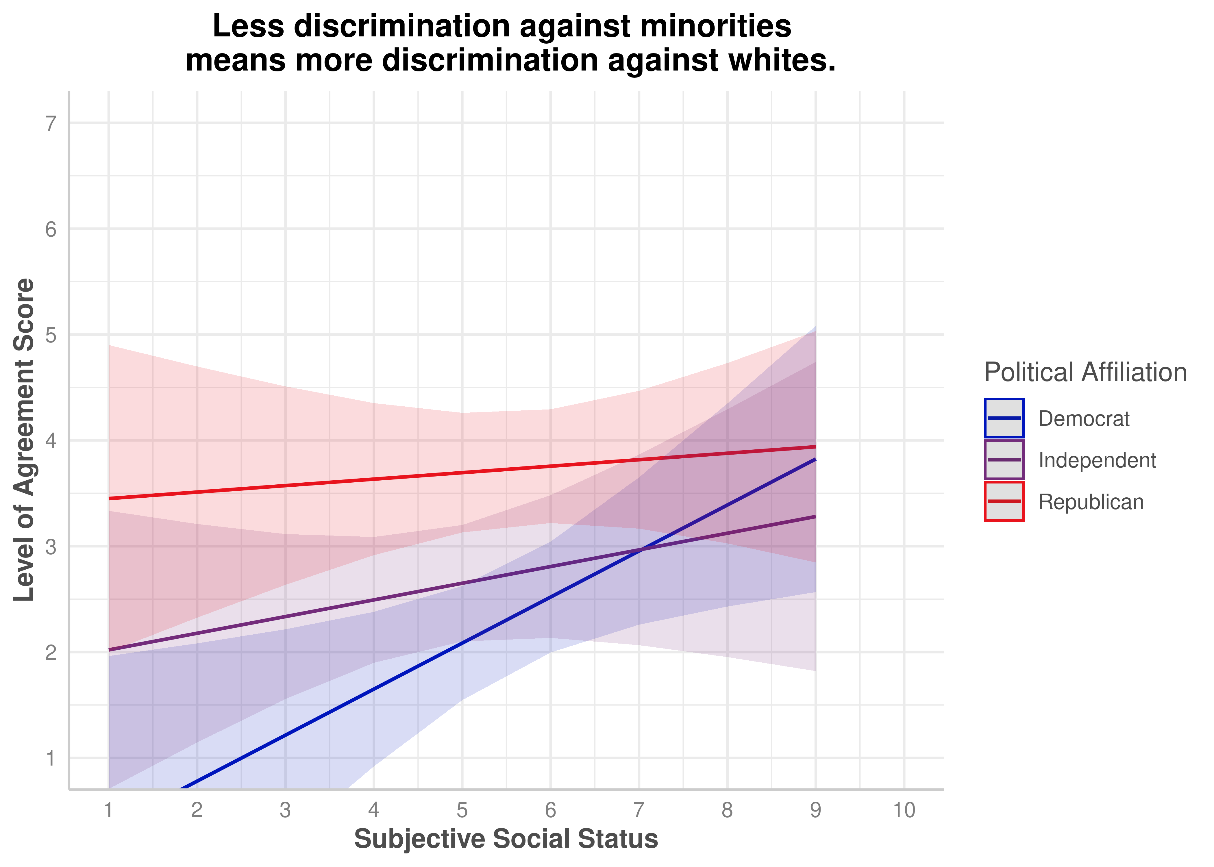
ZEROSUM_5
Less discrimination against minorities means more discrimination against whites.
No
.139
ZEROSUM_6
More opportunity for transwomen means less opportunity for people assigned female at birth.
Yes, p < .001
.212
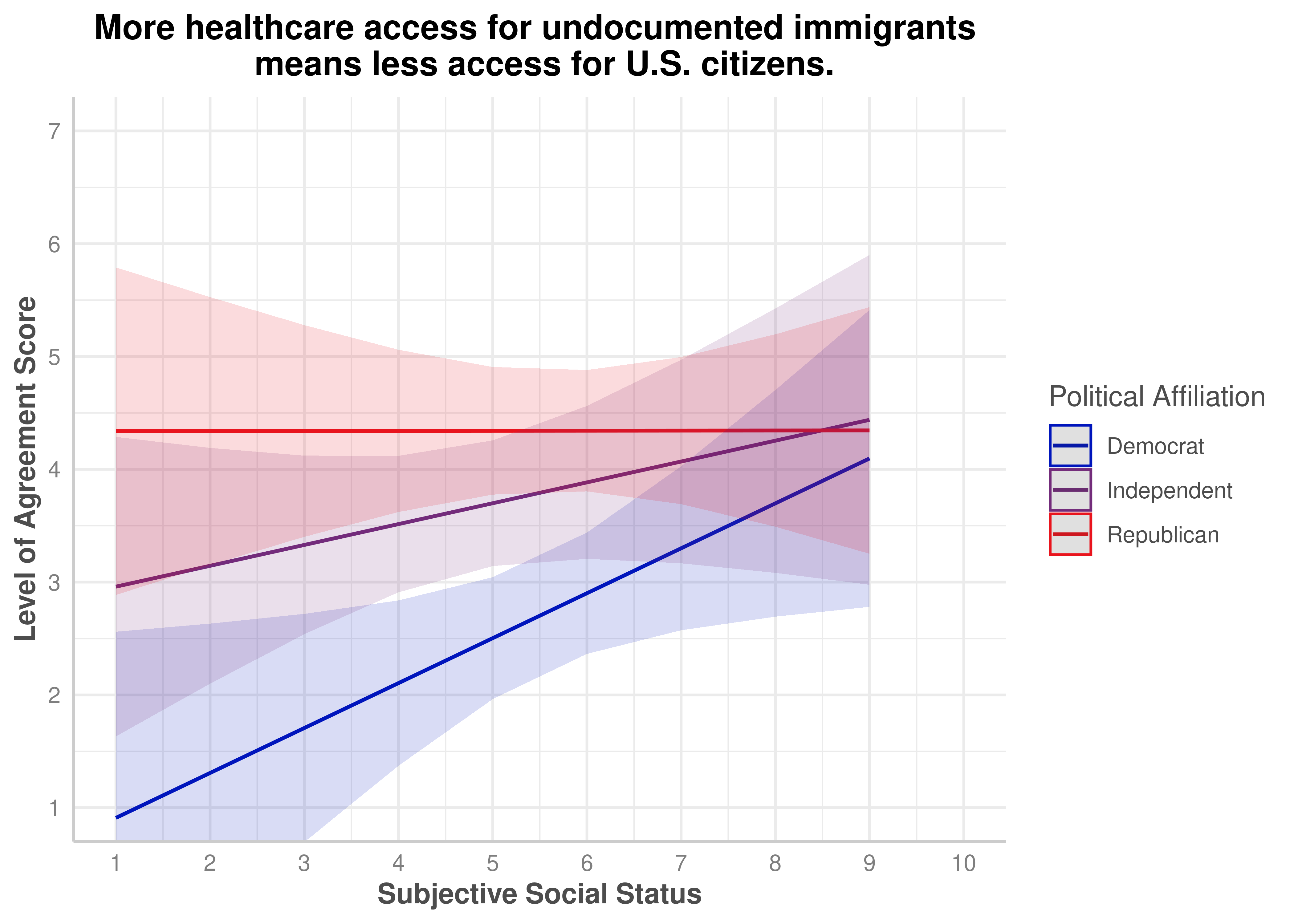
ZEROSUM_7
More healthcare access for undocumented immigrants means less access for U.S. citizens.
No
.157
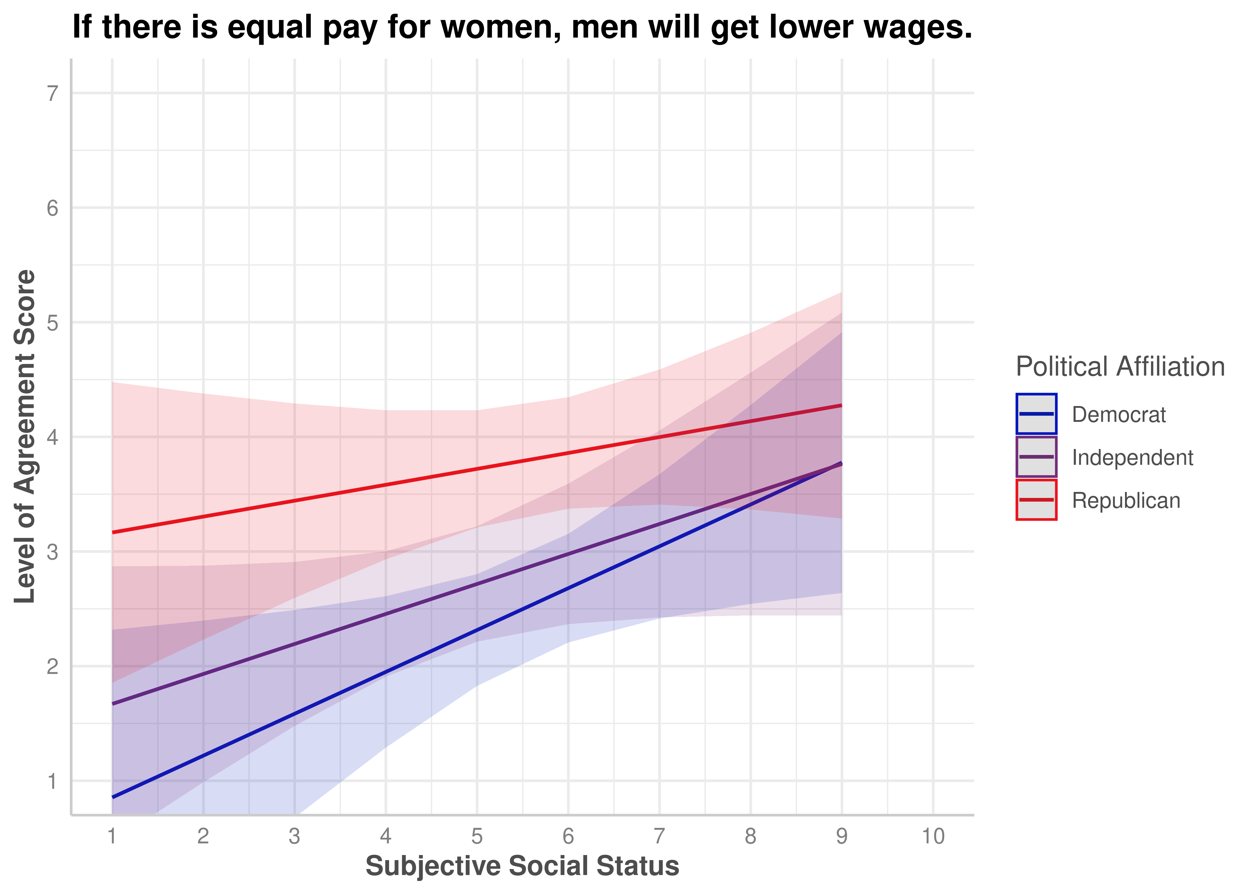
ZEROSUM_8
If there is equal pay for women, men will get lower wages.
No
.165
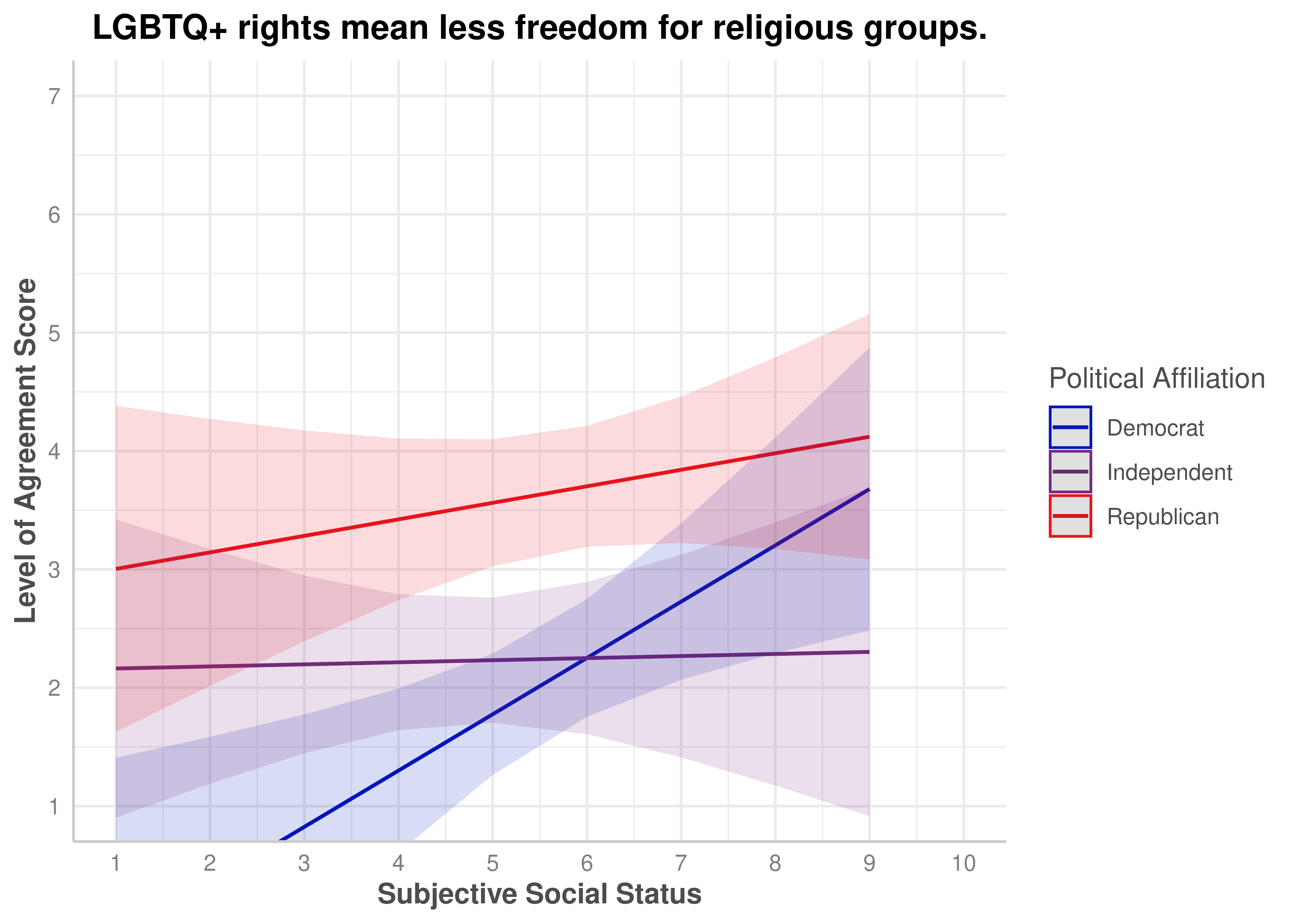
ZEROSUM_9
LGBTQ+ rights mean less freedom for religious groups.
Yes, p < .001
.204
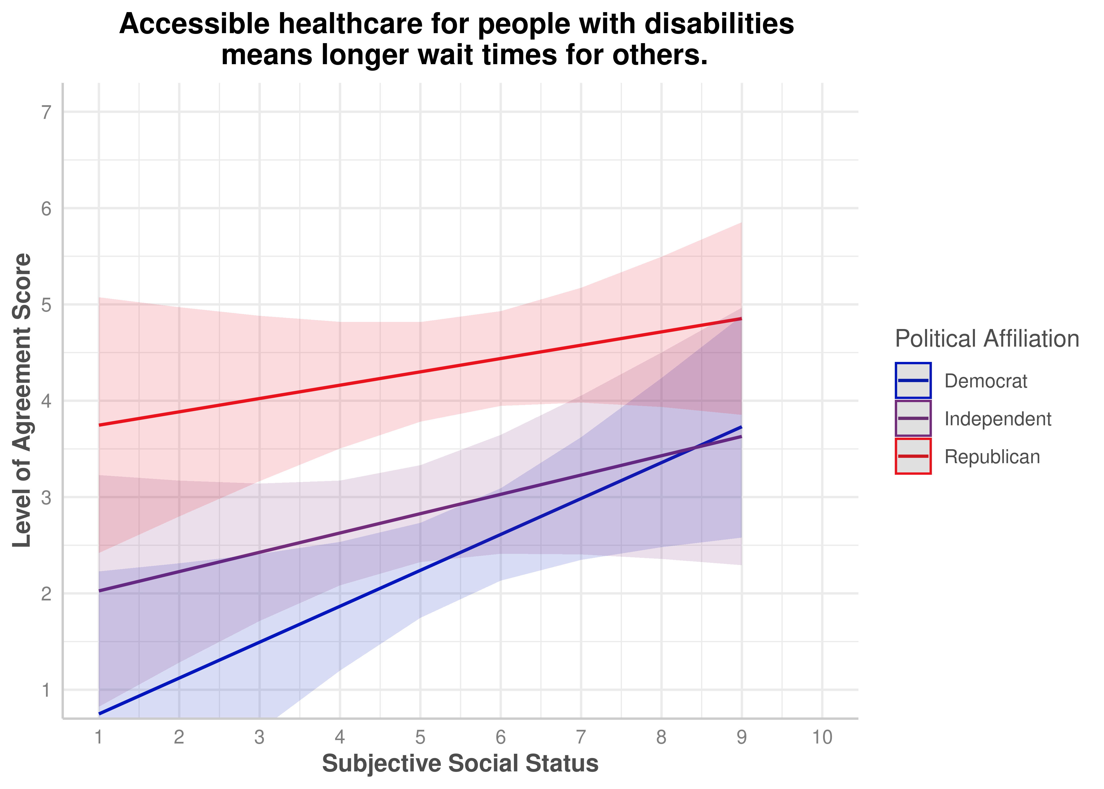
ZEROSUM_10
Accessible healthcare for people with disabilities means longer wait times for others.
No
.262
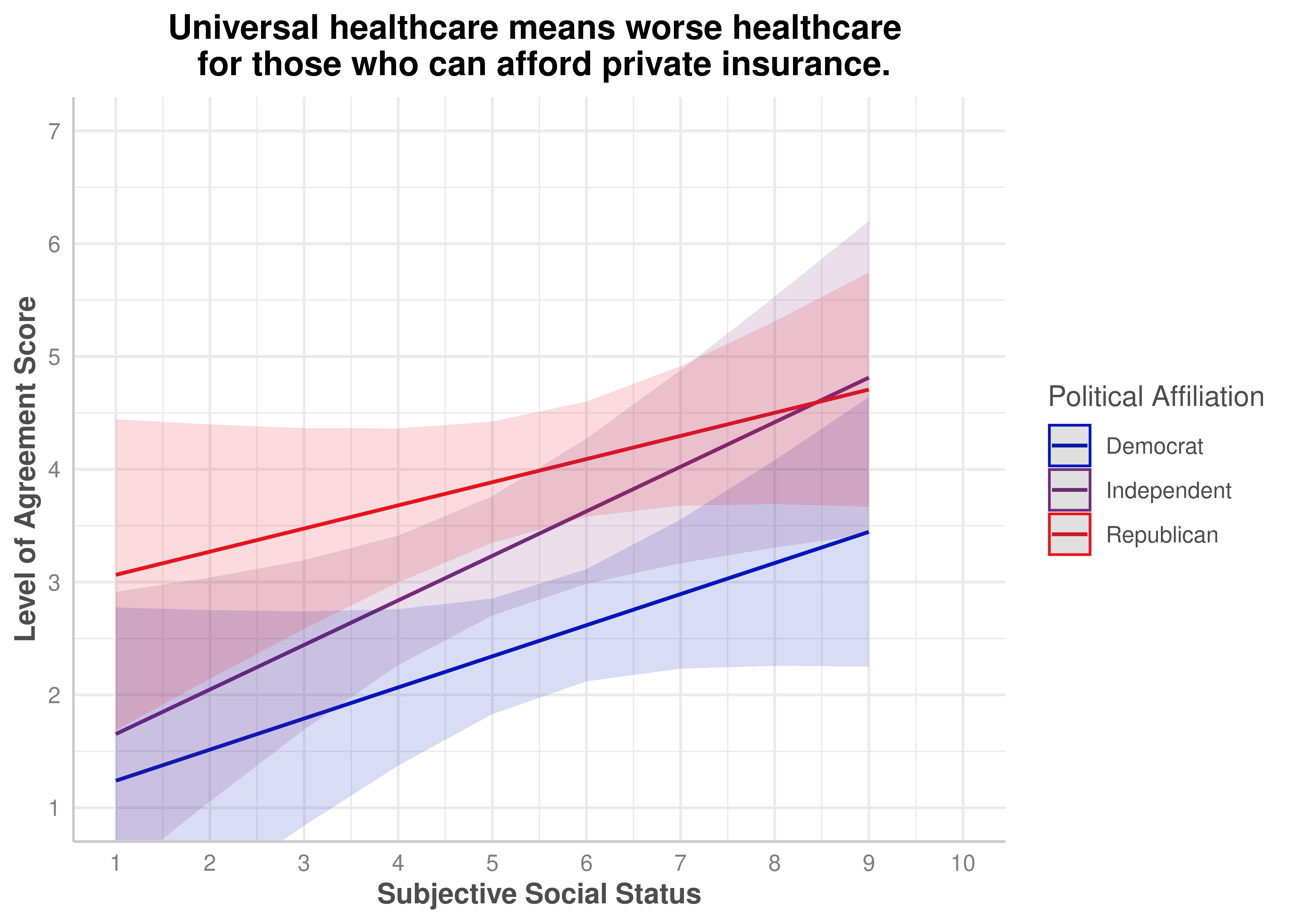
ZEROSUM_11
Universal healthcare means worse healthcare for those who can afford private insurance.
No
.185
Note. Bold text indicates statistically significant SOCIALSTATUS × POLITICALPARTY interaction (p < .05). R² from lm() summary output.
Two-Way ANCOVA (Subjective Social Status x Political Party) on Zero-Sum Beliefs
As a supplementary set of exploratory ANCOVAs, subjective social status (SSS; continuous) and political party affiliation (Democrat [reference], Republican, Independent) were entered as predictors along with their two-way interaction for each of the 11 zero-sum belief items.
The four models for which the interaction terms (SSS x Political Party) achieved significance are reported below (ZEROSUM_3, ZEROSUM_4, ZEROSUM_6, ZEROSUM_9). For these models, SSS consistently functioned as a significant linear predictor, and political party intercept differences and interaction terms revealed meaningful moderation patterns that are described and visualized in the predicted marginal means plots (see appendix B).
ZEROSUM_3: The Wealth of the Few Is Acquired at the Expense of Many
The overall ANCOVA model for ZEROSUM_3 was statistically significant, F(5, 109) = 4.06, p = .002, R-squared = .157, indicating that the model explained approximately 15.7% of variance in endorsement of this economic zero-sum belief.
Among individual predictors, SSS was a significant negative predictor for Democrats, b = −0.39, SE = 0.15, t(109) = −2.66, p = .009, indicating that higher status Democrats endorsed this belief less strongly. Republicans differed significantly from Democrats at the intercept, b = −2.49, SE = 1.12, t(109) = −2.22, p = .029, reflecting lower predicted ZEROSUM_3 scores for Republicans at low SSS values. The SSS x Republican interaction approached significance, b = 0.36, SE = 0.19, t(109) = 1.90, p = .059, suggesting a trend toward a flatter SSS slope for Republicans relative to Democrats.
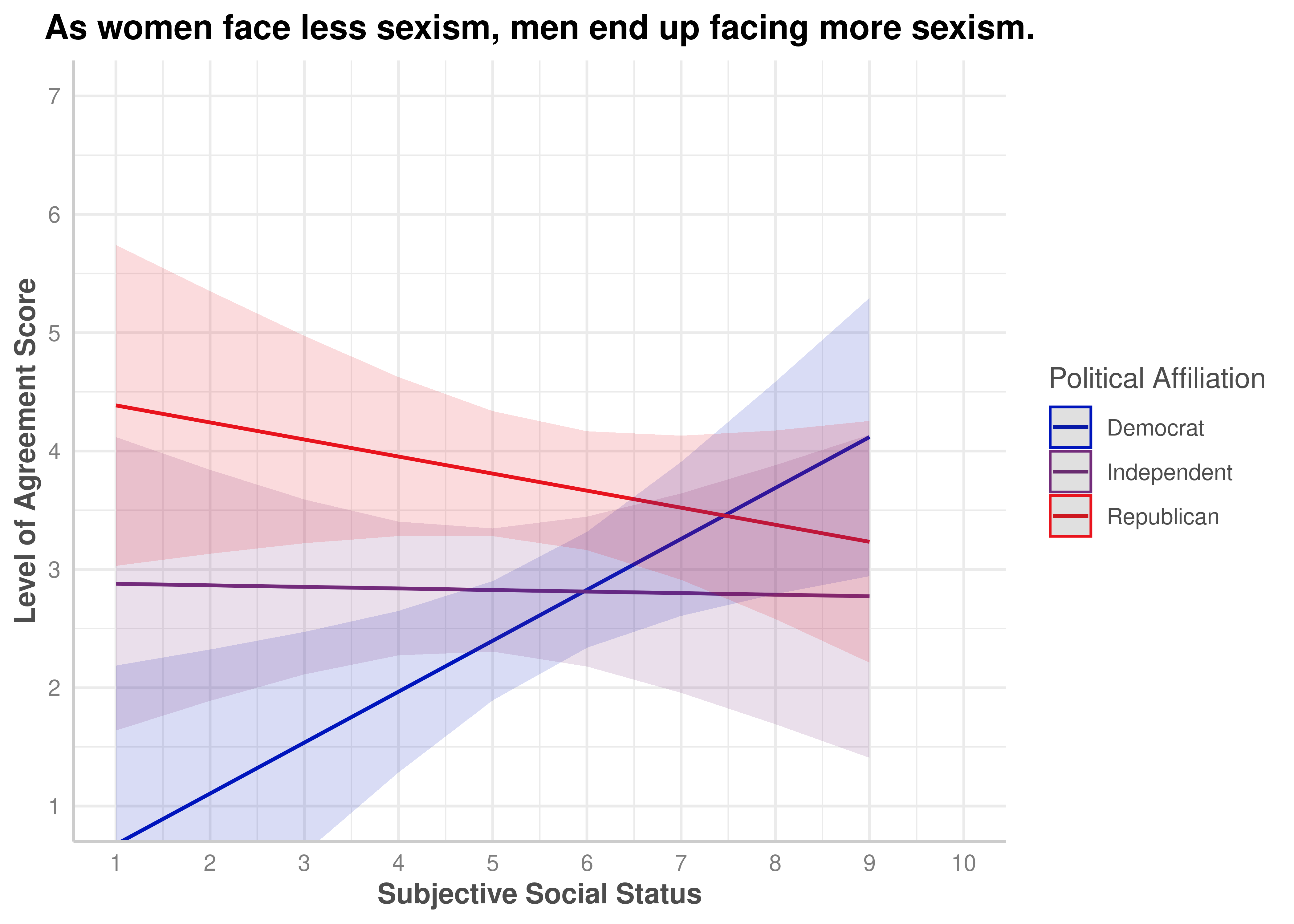
ZEROSUM_4: Reduced Sexism Against Women Implies More Sexism Against Men
The overall ANCOVA model for ZEROSUM_4 was statistically significant, F(5, 109) = 3.83, p = .003, R-squared = .149, explaining approximately 14.9% of variance.
Among individual predictors, SSS was a significant positive predictor for Democrats, b = 0.43, SE = 0.16, t(109) = 2.71, p = .008, indicating that higher status Democrats were more likely to endorse gender-based zero-sum beliefs. Republicans differed significantly from Democrats at the intercept, b = 4.28, SE = 1.22, t(109) = 3.50, p < .001, and Independents also differed from Democrats at the intercept, b = 2.65, SE = 1.19, t(109) = 2.22, p = .029. Critically, both interaction terms were significant: SSS x Independent, b = −0.44, SE = 0.22, t(109) = −2.03, p = .045, and SSS x Republican, b = −0.57, SE = 0.21, t(109) = −2.75, p = .007.
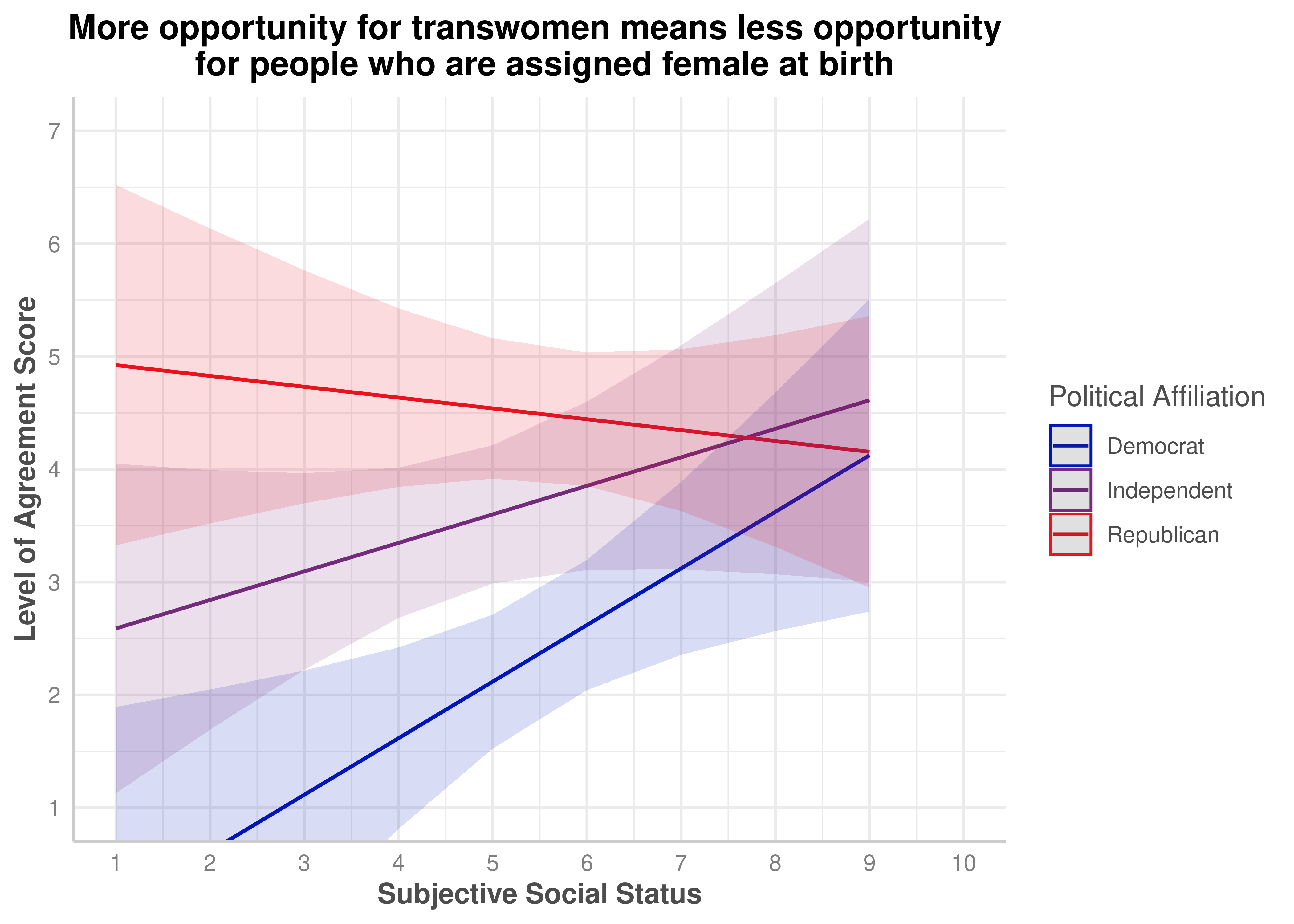
ZEROSUM_6: More Opportunity for Transwomen Means Less Opportunity for Cisgender Women
The overall ANCOVA model for ZEROSUM_6 was statistically significant, F(5, 109) = 7.14, p < .001, R-squared = .247, explaining approximately 24.7% of variance.
Among individual predictors, SSS was a significant positive predictor for Democrats, b = 0.50, SE = 0.19, t(109) = 2.68, p = .008. Republicans differed from Democrats at the intercept, b = 5.41, SE = 1.44, t(109) = 3.75, p < .001, reflecting substantially higher ZEROSUM_6 scores for Republicans at low SSS. The Independent vs. Democrat intercept difference approached significance, b = 2.73, SE = 1.41, t(109) = 1.94, p = .055. The SSS x Republican interaction was significant, b = −0.60, SE = 0.25, t(109) = −2.43, p = .017.
ZEROSUM_9: LGBTQ+ Rights Mean Less Freedom for Religious Groups
The overall ANCOVA model for ZEROSUM_9 was highly significant, F(5, 109) = 6.86, p < .001, R-squared = .239, explaining approximately 23.9% of variance.
Among individual predictors, SSS was a significant positive predictor for Democrats, b = 0.48, SE = 0.16, t(109) = 2.95, p = .004. Republicans differed significantly from Democrats at the intercept, b = 3.47, SE = 1.24, t(109) = 2.79, p = .006, and Independents also differed, b = 2.75, SE = 1.21, t(109) = 2.27, p = .025. The SSS x Independent interaction was significant, b = −0.46, SE = 0.22, t(109) = −2.06, p = .042, while the SSS x Republican interaction was not significant, b = −0.34, SE = 0.21, t(109) = −1.58, p = .116.
Two-way ANCOVA (only SSS)
In [1]:
Show the code
# Run install.R to ensure packages are installedsource("install.R")
Attaching package: 'dplyr'
The following objects are masked from 'package:stats':

    filter, lag
The following objects are masked from 'package:base':

    intersect, setdiff, setequal, union
Registered S3 methods overwritten by 'ggpp':
  method                  from
  heightDetails.titleGrob ggplot2
  widthDetails.titleGrob  ggplot2
Attaching package: 'codebook'
The following object is masked from 'package:codebookr':

    codebook
Suggested APA citation: Thériault, R. (2023). rempsyc: Convenience functions for psychology.
Journal of Open Source Software, 8(87), 5466. https://doi.org/10.21105/joss.05466
Loading required package: carData
Attaching package: 'car'
The following object is masked from 'package:dplyr':

    recode
Attaching package: 'dataMaid'
The following object is masked from 'package:rmarkdown':

    render
The following object is masked from 'package:dplyr':

    summarize
Loading required package: usethis
Attaching package: 'devtools'
The following object is masked from 'package:dataMaid':

    check
Attaching package: 'psych'
The following object is masked from 'package:MBESS':

    cor2cov
The following object is masked from 'package:car':

    logit
The following object is masked from 'package:codebook':

    bfi
The following objects are masked from 'package:ggplot2':

    %+%, alpha
corrplot 0.95 loaded
Loading required package: rpart
randomForest 4.7-1.2
Type rfNews() to see new features/changes/bug fixes.
Attaching package: 'randomForest'
The following object is masked from 'package:psych':

    outlier
The following object is masked from 'package:dplyr':

    combine
The following object is masked from 'package:ggplot2':

    margin
Some of the focal terms are of type `character`. This may lead to
unexpected results. It is recommended to convert these variables to
factors before fitting the model.
The following variables are of type character: `POLITICALPARTY`
Show the code
zerosum1_social_plot$group <-factor( zerosum1_social_plot$group,levels =c("Democrat", "Independent", "Republican"))plot(zerosum1_social_plot) +scale_color_manual(values = party_colors) +scale_fill_manual(values = party_colors) +scale_x_continuous(breaks =1:10, limits =c(1, 10)) +scale_y_continuous(breaks =1:7) +coord_cartesian(xlim =c(1, 10), ylim =c(1, 7)) +labs(title ="Life is so devised that when somebody gains, others have to lose.",x ="Subjective Social Status",y ="Level of Agreement Score",color ="Political Affiliation" ) +theme(plot.title =element_text(face ="bold", hjust =0.5),axis.title.x =element_text(face ="bold"),axis.title.y =element_text(face ="bold") )
Scale for colour is already present.
Adding another scale for colour, which will replace the existing scale.
Scale for y is already present.
Adding another scale for y, which will replace the existing scale.
ZEROSUM_2:
In [10]:
Show the code
zerosum2_social <-lm(ZEROSUM_2 ~ SOCIALSTATUS * POLITICALPARTY, data = select_data)summary(zerosum2_social)
Call:
lm(formula = ZEROSUM_2 ~ SOCIALSTATUS * POLITICALPARTY, data = select_data)
Residuals:
Min 1Q Median 3Q Max
-4.1742 -1.0303 -0.0591 0.9553 2.7254
Coefficients:
Estimate Std. Error t value Pr(>|t|)
(Intercept) 5.23182 0.95105 5.501 2.52e-07 ***
SOCIALSTATUS -0.02879 0.16484 -0.175 0.862
POLITICALPARTYIndependent 0.75995 1.24002 0.613 0.541
POLITICALPARTYRepublican -1.09142 1.27184 -0.858 0.393
SOCIALSTATUS:POLITICALPARTYIndependent -0.24494 0.22753 -1.077 0.284
SOCIALSTATUS:POLITICALPARTYRepublican 0.07353 0.21716 0.339 0.736
---
Signif. codes: 0 '***' 0.001 '**' 0.01 '*' 0.05 '.' 0.1 ' ' 1
Residual standard error: 1.601 on 109 degrees of freedom
(1 observation deleted due to missingness)
Multiple R-squared: 0.05857, Adjusted R-squared: 0.01539
F-statistic: 1.356 on 5 and 109 DF, p-value: 0.2465
Some of the focal terms are of type `character`. This may lead to
unexpected results. It is recommended to convert these variables to
factors before fitting the model.
The following variables are of type character: `POLITICALPARTY`
Show the code
zerosum2_social_plot$group <-factor( zerosum2_social_plot$group,levels =c("Democrat", "Independent", "Republican"))plot(zerosum2_social_plot) +scale_color_manual(values = party_colors) +scale_fill_manual(values = party_colors) +scale_x_continuous(breaks =1:10, limits =c(1, 10)) +scale_y_continuous(breaks =1:7) +coord_cartesian(xlim =c(1, 10), ylim =c(1, 7)) +labs(title ="When some people are getting poorer, \n it means that other people are getting richer.",x ="Subjective Social Status",y ="Level of Agreement Score",color ="Political Affiliation" ) +theme(plot.title =element_text(face ="bold", hjust =0.5),axis.title.x =element_text(face ="bold"),axis.title.y =element_text(face ="bold") )
Scale for colour is already present.
Adding another scale for colour, which will replace the existing scale.
Scale for y is already present.
Adding another scale for y, which will replace the existing scale.
ZEROSUM_3:
In [12]:
Show the code
zerosum3_social <-lm(ZEROSUM_3 ~ SOCIALSTATUS * POLITICALPARTY, data = select_data)summary(zerosum3_social)
Call:
lm(formula = ZEROSUM_3 ~ SOCIALSTATUS * POLITICALPARTY, data = select_data)
Residuals:
Min 1Q Median 3Q Max
-4.3636 -0.7426 0.3044 0.9432 2.3444
Coefficients:
Estimate Std. Error t value Pr(>|t|)
(Intercept) 7.29545 0.83848 8.701 3.86e-14 ***
SOCIALSTATUS -0.38636 0.14533 -2.658 0.00903 **
POLITICALPARTYIndependent -0.31520 1.09324 -0.288 0.77365
POLITICALPARTYRepublican -2.48757 1.12130 -2.218 0.02860 *
SOCIALSTATUS:POLITICALPARTYIndependent -0.07058 0.20060 -0.352 0.72564
SOCIALSTATUS:POLITICALPARTYRepublican 0.36461 0.19145 1.904 0.05949 .
---
Signif. codes: 0 '***' 0.001 '**' 0.01 '*' 0.05 '.' 0.1 ' ' 1
Residual standard error: 1.411 on 109 degrees of freedom
(1 observation deleted due to missingness)
Multiple R-squared: 0.1571, Adjusted R-squared: 0.1185
F-statistic: 4.064 on 5 and 109 DF, p-value: 0.002021
Some of the focal terms are of type `character`. This may lead to
unexpected results. It is recommended to convert these variables to
factors before fitting the model.
The following variables are of type character: `POLITICALPARTY`
Show the code
zerosum3_social_plot$group <-factor( zerosum3_social_plot$group,levels =c("Democrat", "Independent", "Republican"))plot(zerosum3_social_plot) +geom_point(data = select_data,aes(x = SOCIALSTATUS, y = ZEROSUM_3, color = POLITICALPARTY),alpha =0.3,size =1.5,position =position_jitter(width =0.45, height =0.4),inherit.aes =FALSE ) +scale_color_manual(values = party_colors) +scale_fill_manual(values = party_colors) +scale_x_continuous(breaks =1:10, limits =c(1, 10)) +scale_y_continuous(breaks =1:7) +coord_cartesian(xlim =c(1, 10), ylim =c(1, 7)) +labs(title ="The wealth of a few is acquired at the expense of many.",x ="Subjective Social Status",y ="Level of Agreement Score",color ="Political Affiliation" ) +theme(plot.title =element_text(face ="bold", hjust =0.5),axis.title.x =element_text(face ="bold"),axis.title.y =element_text(face ="bold") )
Scale for colour is already present.
Adding another scale for colour, which will replace the existing scale.
Scale for y is already present.
Adding another scale for y, which will replace the existing scale.
Warning: Removed 3 rows containing missing values or values outside the scale range
(`geom_point()`).
ZEROSUM_4:
In [14]:
Show the code
zerosum4_social <-lm(ZEROSUM_4 ~ SOCIALSTATUS * POLITICALPARTY, data = select_data)summary(zerosum4_social)
Call:
lm(formula = ZEROSUM_4 ~ SOCIALSTATUS * POLITICALPARTY, data = select_data)
Residuals:
Min 1Q Median 3Q Max
-2.9532 -1.3970 -0.0973 1.1736 3.4636
Coefficients:
Estimate Std. Error t value Pr(>|t|)
(Intercept) 0.2455 0.9146 0.268 0.788927
SOCIALSTATUS 0.4303 0.1585 2.714 0.007723 **
POLITICALPARTYIndependent 2.6459 1.1925 2.219 0.028577 *
POLITICALPARTYRepublican 4.2841 1.2231 3.503 0.000669 ***
SOCIALSTATUS:POLITICALPARTYIndependent -0.4435 0.2188 -2.027 0.045137 *
SOCIALSTATUS:POLITICALPARTYRepublican -0.5744 0.2088 -2.750 0.006972 **
---
Signif. codes: 0 '***' 0.001 '**' 0.01 '*' 0.05 '.' 0.1 ' ' 1
Residual standard error: 1.539 on 109 degrees of freedom
(1 observation deleted due to missingness)
Multiple R-squared: 0.1495, Adjusted R-squared: 0.1105
F-statistic: 3.831 on 5 and 109 DF, p-value: 0.003093
Some of the focal terms are of type `character`. This may lead to
unexpected results. It is recommended to convert these variables to
factors before fitting the model.
The following variables are of type character: `POLITICALPARTY`
Show the code
zerosum4_social_plot$group <-factor( zerosum4_social_plot$group,levels =c("Democrat", "Independent", "Republican"))plot(zerosum4_social_plot) +scale_color_manual(values = party_colors) +scale_fill_manual(values = party_colors) +scale_x_continuous(breaks =1:10, limits =c(1, 10)) +scale_y_continuous(breaks =1:7) +coord_cartesian(xlim =c(1, 10), ylim =c(1, 7)) +labs(title ="As women face less sexism, men end up facing more sexism.",x ="Subjective Social Status",y ="Level of Agreement Score",color ="Political Affiliation" )+theme(plot.title =element_text(face ="bold", hjust =0.5),axis.title.x =element_text(face ="bold"),axis.title.y =element_text(face ="bold") )
Scale for colour is already present.
Adding another scale for colour, which will replace the existing scale.
Scale for y is already present.
Adding another scale for y, which will replace the existing scale.
ZEROSUM_5:
In [16]:
Show the code
zerosum5_social <-lm(ZEROSUM_5 ~ SOCIALSTATUS * POLITICALPARTY, data = select_data)summary(zerosum5_social)
Call:
lm(formula = ZEROSUM_5 ~ SOCIALSTATUS * POLITICALPARTY, data = select_data)
Residuals:
Min 1Q Median 3Q Max
-2.8173 -1.1475 -0.4412 1.3495 4.3495
Coefficients:
Estimate Std. Error t value Pr(>|t|)
(Intercept) -0.08939 0.97853 -0.091 0.92738
SOCIALSTATUS 0.43485 0.16961 2.564 0.01170 *
POLITICALPARTYIndependent 1.95230 1.27164 1.535 0.12759
POLITICALPARTYRepublican 3.47856 1.30859 2.658 0.00903 **
SOCIALSTATUS:POLITICALPARTYIndependent -0.27733 0.23379 -1.186 0.23809
SOCIALSTATUS:POLITICALPARTYRepublican -0.37368 0.22343 -1.672 0.09727 .
---
Signif. codes: 0 '***' 0.001 '**' 0.01 '*' 0.05 '.' 0.1 ' ' 1
Residual standard error: 1.647 on 110 degrees of freedom
Multiple R-squared: 0.1765, Adjusted R-squared: 0.1391
F-statistic: 4.716 on 5 and 110 DF, p-value: 0.0006099
Some of the focal terms are of type `character`. This may lead to
unexpected results. It is recommended to convert these variables to
factors before fitting the model.
The following variables are of type character: `POLITICALPARTY`
Show the code
zerosum5_social_plot$group <-factor( zerosum5_social_plot$group,levels =c("Democrat", "Independent", "Republican"))plot(zerosum5_social_plot) +scale_color_manual(values = party_colors) +scale_fill_manual(values = party_colors) +scale_x_continuous(breaks =1:10, limits =c(1, 10)) +scale_y_continuous(breaks =1:7) +coord_cartesian(xlim =c(1, 10), ylim =c(1, 7)) +labs(title ="Less discrimination against minorities \n means more discrimination against whites.",x ="Subjective Social Status",y ="Level of Agreement Score",color ="Political Affiliation" ) +theme(plot.title =element_text(face ="bold", hjust =0.5),axis.title.x =element_text(face ="bold"),axis.title.y =element_text(face ="bold") )
Scale for colour is already present.
Adding another scale for colour, which will replace the existing scale.
Scale for y is already present.
Adding another scale for y, which will replace the existing scale.
ZEROSUM_6:
In [18]:
Show the code
zerosum6_social <-lm(ZEROSUM_6 ~ SOCIALSTATUS * POLITICALPARTY, data = select_data)summary(zerosum6_social)
Call:
lm(formula = ZEROSUM_6 ~ SOCIALSTATUS * POLITICALPARTY, data = select_data)
Residuals:
Min 1Q Median 3Q Max
-3.6355 -1.5891 -0.1152 1.4780 3.6522
Coefficients:
Estimate Std. Error t value Pr(>|t|)
(Intercept) -0.3894 1.0779 -0.361 0.718605
SOCIALSTATUS 0.5015 0.1868 2.684 0.008401 **
POLITICALPARTYIndependent 2.7257 1.4054 1.939 0.055032 .
POLITICALPARTYRepublican 5.4091 1.4415 3.753 0.000282 ***
SOCIALSTATUS:POLITICALPARTYIndependent -0.2486 0.2579 -0.964 0.337085
SOCIALSTATUS:POLITICALPARTYRepublican -0.5976 0.2461 -2.428 0.016819 *
---
Signif. codes: 0 '***' 0.001 '**' 0.01 '*' 0.05 '.' 0.1 ' ' 1
Residual standard error: 1.814 on 109 degrees of freedom
(1 observation deleted due to missingness)
Multiple R-squared: 0.2468, Adjusted R-squared: 0.2123
F-statistic: 7.143 on 5 and 109 DF, p-value: 8.149e-06
Some of the focal terms are of type `character`. This may lead to
unexpected results. It is recommended to convert these variables to
factors before fitting the model.
The following variables are of type character: `POLITICALPARTY`
Show the code
zerosum6_social_plot$group <-factor( zerosum6_social_plot$group,levels =c("Democrat", "Independent", "Republican"))plot(zerosum6_social_plot) +scale_color_manual(values = party_colors) +scale_fill_manual(values = party_colors) +scale_x_continuous(breaks =1:10, limits =c(1,10)) +scale_y_continuous(breaks =1:7) +coord_cartesian(xlim =c(1, 10), ylim =c(1, 7)) +labs(title ="More opportunity for transwomen means less opportunity \n for people who are assigned female at birth",x ="Subjective Social Status",y ="Level of Agreement Score",color ="Political Affiliation" )+theme(plot.title =element_text(face ="bold", hjust =0.5),axis.title.x =element_text(face ="bold"),axis.title.y =element_text(face ="bold") )
Scale for colour is already present.
Adding another scale for colour, which will replace the existing scale.
Scale for y is already present.
Adding another scale for y, which will replace the existing scale.
ZEROSUM_7:
In [20]:
Show the code
zerosum7_social <-lm(ZEROSUM_7 ~ SOCIALSTATUS * POLITICALPARTY, data = select_data)summary(zerosum7_social)
Call:
lm(formula = ZEROSUM_7 ~ SOCIALSTATUS * POLITICALPARTY, data = select_data)
Residuals:
Min 1Q Median 3Q Max
-3.3407 -1.3417 0.0984 1.0128 3.8950
Coefficients:
Estimate Std. Error t value Pr(>|t|)
(Intercept) 0.5119 1.0008 0.511 0.61005
SOCIALSTATUS 0.3983 0.1754 2.270 0.02519 *
POLITICALPARTYIndependent 2.2632 1.2934 1.750 0.08299 .
POLITICALPARTYRepublican 3.8256 1.3257 2.886 0.00472 **
SOCIALSTATUS:POLITICALPARTYIndependent -0.2134 0.2385 -0.895 0.37275
SOCIALSTATUS:POLITICALPARTYRepublican -0.3975 0.2280 -1.744 0.08409 .
---
Signif. codes: 0 '***' 0.001 '**' 0.01 '*' 0.05 '.' 0.1 ' ' 1
Residual standard error: 1.648 on 108 degrees of freedom
(2 observations deleted due to missingness)
Multiple R-squared: 0.1947, Adjusted R-squared: 0.1574
F-statistic: 5.221 on 5 and 108 DF, p-value: 0.000248
Some of the focal terms are of type `character`. This may lead to
unexpected results. It is recommended to convert these variables to
factors before fitting the model.
The following variables are of type character: `POLITICALPARTY`
Show the code
zerosum7_social_plot$group <-factor( zerosum7_social_plot$group,levels =c("Democrat", "Independent", "Republican"))plot(zerosum7_social_plot) +scale_color_manual(values = party_colors) +scale_fill_manual(values = party_colors) +scale_x_continuous(breaks =1:10, limits =c(1, 10)) +scale_y_continuous(breaks =1:7) +coord_cartesian(xlim =c(1, 10), ylim =c(1, 7)) +labs(title ="More healthcare access for undocumented immigrants \n means less access for U.S. citizens.",x ="Subjective Social Status",y ="Level of Agreement Score",color ="Political Affiliation" ) +theme(plot.title =element_text(face ="bold", hjust =0.5),axis.title.x =element_text(face ="bold"),axis.title.y =element_text(face ="bold") )
Scale for colour is already present.
Adding another scale for colour, which will replace the existing scale.
Scale for y is already present.
Adding another scale for y, which will replace the existing scale.
ZEROSUM_8:
In [22]:
Show the code
zerosum8_social <-lm(ZEROSUM_8 ~ SOCIALSTATUS * POLITICALPARTY, data = select_data)summary(zerosum8_social)
Call:
lm(formula = ZEROSUM_8 ~ SOCIALSTATUS * POLITICALPARTY, data = select_data)
Residuals:
Min 1Q Median 3Q Max
-2.9984 -1.1654 0.0016 1.0500 3.5567
Coefficients:
Estimate Std. Error t value Pr(>|t|)
(Intercept) 0.4894 0.8851 0.553 0.5815
SOCIALSTATUS 0.3652 0.1534 2.380 0.0190 *
POLITICALPARTYIndependent 0.9193 1.1541 0.797 0.4274
POLITICALPARTYRepublican 2.5377 1.1837 2.144 0.0343 *
SOCIALSTATUS:POLITICALPARTYIndependent -0.1035 0.2118 -0.489 0.6260
SOCIALSTATUS:POLITICALPARTYRepublican -0.2264 0.2021 -1.120 0.2651
---
Signif. codes: 0 '***' 0.001 '**' 0.01 '*' 0.05 '.' 0.1 ' ' 1
Residual standard error: 1.49 on 109 degrees of freedom
(1 observation deleted due to missingness)
Multiple R-squared: 0.2016, Adjusted R-squared: 0.165
F-statistic: 5.505 on 5 and 109 DF, p-value: 0.0001474
Some of the focal terms are of type `character`. This may lead to
unexpected results. It is recommended to convert these variables to
factors before fitting the model.
The following variables are of type character: `POLITICALPARTY`
Show the code
zerosum8_social_plot$group <-factor( zerosum8_social_plot$group,levels =c("Democrat", "Independent", "Republican"))plot(zerosum8_social_plot) +scale_color_manual(values = party_colors) +scale_fill_manual(values = party_colors) +scale_x_continuous(breaks =1:10, limits =c(1, 10)) +scale_y_continuous(breaks =1:7) +coord_cartesian(xlim =c(1, 10), ylim =c(1, 7)) +labs(title ="If there is equal pay for women, men will get lower wages.",x ="Subjective Social Status",y ="Level of Agreement Score",color ="Political Affiliation" ) +theme(plot.title =element_text(face ="bold", hjust =0.5),axis.title.x =element_text(face ="bold"),axis.title.y =element_text(face ="bold") )
Scale for colour is already present.
Adding another scale for colour, which will replace the existing scale.
Scale for y is already present.
Adding another scale for y, which will replace the existing scale.
ZEROSUM_9:
In [24]:
Show the code
zerosum9_social <-lm(ZEROSUM_9 ~ SOCIALSTATUS * POLITICALPARTY, data = select_data)summary(zerosum9_social)
Call:
lm(formula = ZEROSUM_9 ~ SOCIALSTATUS * POLITICALPARTY, data = select_data)
Residuals:
Min 1Q Median 3Q Max
-2.8415 -1.2326 -0.2515 1.2485 3.7850
Coefficients:
Estimate Std. Error t value Pr(>|t|)
(Intercept) -0.6030 0.9295 -0.649 0.51785
SOCIALSTATUS 0.4758 0.1611 2.953 0.00386 **
POLITICALPARTYIndependent 2.7478 1.2119 2.267 0.02534 *
POLITICALPARTYRepublican 3.4676 1.2430 2.790 0.00623 **
SOCIALSTATUS:POLITICALPARTYIndependent -0.4582 0.2224 -2.061 0.04173 *
SOCIALSTATUS:POLITICALPARTYRepublican -0.3362 0.2122 -1.584 0.11609
---
Signif. codes: 0 '***' 0.001 '**' 0.01 '*' 0.05 '.' 0.1 ' ' 1
Residual standard error: 1.564 on 109 degrees of freedom
(1 observation deleted due to missingness)
Multiple R-squared: 0.2393, Adjusted R-squared: 0.2044
F-statistic: 6.857 on 5 and 109 DF, p-value: 1.342e-05
Some of the focal terms are of type `character`. This may lead to
unexpected results. It is recommended to convert these variables to
factors before fitting the model.
The following variables are of type character: `POLITICALPARTY`
Show the code
zerosum9_social_plot$group <-factor( zerosum9_social_plot$group,levels =c("Democrat", "Independent", "Republican"))plot(zerosum9_social_plot) +scale_color_manual(values = party_colors) +scale_fill_manual(values = party_colors) +scale_x_continuous(breaks =1:10, limits =c(1,10)) +scale_y_continuous(breaks =1:7) +coord_cartesian(xlim =c(1, 10), ylim =c(1, 7)) +labs(title ="LGBTQ+ rights mean less freedom for religious groups.",x ="Subjective Social Status",y ="Level of Agreement Score",color ="Political Affiliation" )+theme(plot.title =element_text(face ="bold", hjust =0.5),axis.title.x =element_text(face ="bold"),axis.title.y =element_text(face ="bold") )
Scale for colour is already present.
Adding another scale for colour, which will replace the existing scale.
Scale for y is already present.
Adding another scale for y, which will replace the existing scale.
ZEROSUM_10:
In [26]:
Show the code
zerosum10_social <-lm(ZEROSUM_10 ~ SOCIALSTATUS * POLITICALPARTY, data = select_data)summary(zerosum10_social)
Call:
lm(formula = ZEROSUM_10 ~ SOCIALSTATUS * POLITICALPARTY, data = select_data)
Residuals:
Min 1Q Median 3Q Max
-3.5768 -1.2394 -0.0234 1.1529 3.3879
Coefficients:
Estimate Std. Error t value Pr(>|t|)
(Intercept) 0.3758 0.8956 0.420 0.67564
SOCIALSTATUS 0.3727 0.1552 2.401 0.01803 *
POLITICALPARTYIndependent 1.4498 1.1639 1.246 0.21556
POLITICALPARTYRepublican 3.2326 1.1977 2.699 0.00805 **
SOCIALSTATUS:POLITICALPARTYIndependent -0.1722 0.2140 -0.805 0.42258
SOCIALSTATUS:POLITICALPARTYRepublican -0.2344 0.2045 -1.146 0.25423
---
Signif. codes: 0 '***' 0.001 '**' 0.01 '*' 0.05 '.' 0.1 ' ' 1
Residual standard error: 1.507 on 110 degrees of freedom
Multiple R-squared: 0.2936, Adjusted R-squared: 0.2615
F-statistic: 9.144 on 5 and 110 DF, p-value: 2.683e-07
Some of the focal terms are of type `character`. This may lead to
unexpected results. It is recommended to convert these variables to
factors before fitting the model.
The following variables are of type character: `POLITICALPARTY`
Show the code
zerosum10_social_plot$group <-factor( zerosum10_social_plot$group,levels =c("Democrat", "Independent", "Republican"))plot(zerosum10_social_plot) +scale_color_manual(values = party_colors) +scale_fill_manual(values = party_colors) +scale_x_continuous(breaks =1:10, limits =c(1, 10)) +scale_y_continuous(breaks =1:7) +coord_cartesian(xlim =c(1, 10), ylim =c(1, 7)) +labs(title ="Accessible healthcare for people with disabilities \n means longer wait times for others.",x ="Subjective Social Status",y ="Level of Agreement Score",color ="Political Affiliation" ) +theme(plot.title =element_text(face ="bold", hjust =0.5),axis.title.x =element_text(face ="bold"),axis.title.y =element_text(face ="bold") )
Scale for colour is already present.
Adding another scale for colour, which will replace the existing scale.
Scale for y is already present.
Adding another scale for y, which will replace the existing scale.
ZEROSUM_11:
In [28]:
Show the code
zerosum11_social <-lm(ZEROSUM_11 ~ SOCIALSTATUS * POLITICALPARTY, data = select_data)summary(zerosum11_social)
Call:
lm(formula = ZEROSUM_11 ~ SOCIALSTATUS * POLITICALPARTY, data = select_data)
Residuals:
Min 1Q Median 3Q Max
-3.2964 -1.3194 -0.0911 1.1855 3.9333
Coefficients:
Estimate Std. Error t value Pr(>|t|)
(Intercept) 0.9636 0.9298 1.036 0.3023
SOCIALSTATUS 0.2758 0.1612 1.711 0.0899 .
POLITICALPARTYIndependent 0.2947 1.2123 0.243 0.8084
POLITICALPARTYRepublican 1.8960 1.2434 1.525 0.1302
SOCIALSTATUS:POLITICALPARTYIndependent 0.1192 0.2225 0.536 0.5932
SOCIALSTATUS:POLITICALPARTYRepublican -0.0705 0.2123 -0.332 0.7405
---
Signif. codes: 0 '***' 0.001 '**' 0.01 '*' 0.05 '.' 0.1 ' ' 1
Residual standard error: 1.565 on 109 degrees of freedom
(1 observation deleted due to missingness)
Multiple R-squared: 0.2204, Adjusted R-squared: 0.1846
F-statistic: 6.163 on 5 and 109 DF, p-value: 4.557e-05
Some of the focal terms are of type `character`. This may lead to
unexpected results. It is recommended to convert these variables to
factors before fitting the model.
The following variables are of type character: `POLITICALPARTY`
Show the code
zerosum11_social_plot$group <-factor( zerosum11_social_plot$group,levels =c("Democrat", "Independent", "Republican"))plot(zerosum11_social_plot) +scale_color_manual(values = party_colors) +scale_fill_manual(values = party_colors) +scale_x_continuous(breaks =1:10, limits =c(1, 10)) +scale_y_continuous(breaks =1:7) +coord_cartesian(xlim =c(1, 10), ylim =c(1, 7)) +labs(title ="Universal healthcare means worse healthcare \n for those who can afford private insurance.",x ="Subjective Social Status",y ="Level of Agreement Score",color ="Political Affiliation" ) +theme(plot.title =element_text(face ="bold", hjust =0.5),axis.title.x =element_text(face ="bold"),axis.title.y =element_text(face ="bold") )
Scale for colour is already present.
Adding another scale for colour, which will replace the existing scale.
Scale for y is already present.
Adding another scale for y, which will replace the existing scale.
Cross-tab table for each SSS with zerosum to see the counts of each political party
In [30]:
Show the code
library(dplyr)library(tidyr)library(knitr)library(kableExtra)table_data <- select_data %>%mutate(POLITICALPARTY =factor( POLITICALPARTY,levels =c("Democrat", "Republican", "Independent") ) ) %>%count(SOCIALSTATUS, POLITICALPARTY) %>%pivot_wider(names_from = POLITICALPARTY,values_from = n,values_fill =0 ) %>%mutate(SOCIALSTATUS =as.character(SOCIALSTATUS))# Add totalstable_data_total <- table_data %>%mutate(Total =rowSums(across(where(is.numeric)), na.rm =TRUE)) %>%bind_rows( table_data %>%summarise(across(where(is.numeric), ~sum(.x, na.rm =TRUE))) %>%mutate(SOCIALSTATUS ="Total",Total =sum(across(where(is.numeric)), na.rm =TRUE) ) )table_data_total %>%kable(caption ="Counts of Political Party within Each Subjective Social Status",align ="c" ) %>%kable_styling(full_width =FALSE, position ="center") %>%row_spec(nrow(table_data_total), bold =TRUE)
Counts of Political Party within Each Subjective Social Status
Warning: Removed 1 row containing non-finite outside the scale range
(`stat_qq()`).
Warning: Removed 1 row containing non-finite outside the scale range
(`stat_qq_line()`).
Warning: Removed 1 row containing non-finite outside the scale range
(`stat_qq()`).
Warning: Removed 1 row containing non-finite outside the scale range
(`stat_qq_line()`).
Warning: Removed 1 row containing non-finite outside the scale range
(`stat_qq()`).
Warning: Removed 1 row containing non-finite outside the scale range
(`stat_qq_line()`).
Warning: Removed 1 row containing non-finite outside the scale range
(`stat_qq()`).
Warning: Removed 1 row containing non-finite outside the scale range
(`stat_qq_line()`).
Warning: Removed 2 rows containing non-finite outside the scale range
(`stat_qq()`).
Warning: Removed 2 rows containing non-finite outside the scale range
(`stat_qq_line()`).
Warning: Removed 1 row containing non-finite outside the scale range
(`stat_qq()`).
Warning: Removed 1 row containing non-finite outside the scale range
(`stat_qq_line()`).
Warning: Removed 1 row containing non-finite outside the scale range
(`stat_qq()`).
Warning: Removed 1 row containing non-finite outside the scale range
(`stat_qq_line()`).
Warning: Removed 1 row containing non-finite outside the scale range
(`stat_qq()`).
Warning: Removed 1 row containing non-finite outside the scale range
(`stat_qq_line()`).
Warning: annotation$theme is not a valid theme.
Please use `theme()` to construct themes.
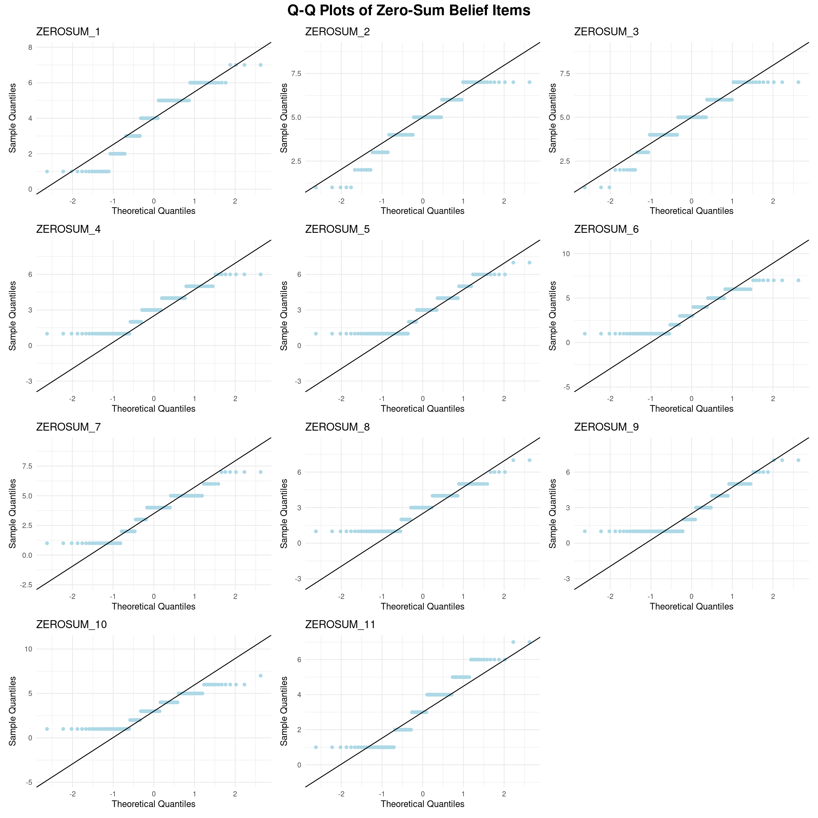
Show the code
## Most of the points are roughly following the diagonal, but many are stepped, this makes sense because ZEROSUM items are Likert-type scores (discrete integers).## the distribution is not perfectly normal, but this is expected for Likert data.
To examine the joint and interactive effects of social identity variables and political party affiliation on zero-sum beliefs, a series of two-way analyses were conducted. For continuous predictors (i.e., subjective social status (SSS)), two-way ANCOVA were used. For categorical predictors (i.e., income, gender, racial identity, and sexual identity), two-way ANOVAs were used. All models included political party affiliation (Democrat, Republican, Independent) as a second factor.
ZEROSUM_1: Social Status x Political Party
In [35]:
Show the code
zerosum1_social <-lm(ZEROSUM_1 ~ SOCIALSTATUS * POLITICALPARTY, data = select_data)summary(zerosum1_social)
Call:
lm(formula = ZEROSUM_1 ~ SOCIALSTATUS * POLITICALPARTY, data = select_data)

Residuals:
    Min      1Q  Median      3Q     Max
-3.4185 -1.2233  0.0246  1.3209  3.3000

Coefficients:
                                       Estimate Std. Error t value Pr(>|t|)
(Intercept)                              3.3500     1.0380   3.227  0.00165 **
SOCIALSTATUS                             0.1167     0.1799   0.648  0.51805
POLITICALPARTYIndependent                1.2689     1.3490   0.941  0.34893
POLITICALPARTYRepublican                 1.0539     1.3882   0.759  0.44933
SOCIALSTATUS:POLITICALPARTYIndependent  -0.3171     0.2480  -1.279  0.20367
SOCIALSTATUS:POLITICALPARTYRepublican   -0.1692     0.2370  -0.714  0.47678
---
Signif. codes:  0 '***' 0.001 '**' 0.01 '*' 0.05 '.' 0.1 ' ' 1

Residual standard error: 1.747 on 110 degrees of freedom
Multiple R-squared:  0.02813,   Adjusted R-squared:  -0.01605
F-statistic: 0.6367 on 5 and 110 DF,  p-value: 0.6721
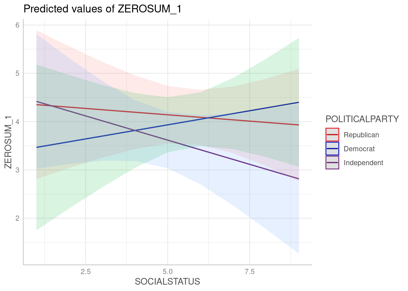
The ANCOVA for ZEROSUM_1 model was not significant, F(5,116) = 1.07, p = 0.3806, R-squared = 0.044. The model explains only ~4.4% of the variance. The relationship between social status and zero-sum beliefs might differ slightly for Independents vs Democrats.
Some of the focal terms are of type `character`. This may lead to
  unexpected results. It is recommended to convert these variables to
  factors before fitting the model.
  The following variables are of type character: `POLITICALPARTY`
Scale for colour is already present.
Adding another scale for colour, which will replace the existing scale.
The interaction term (SSS x Political Party) approached but did not achieve significance (p = .066). It suggests that the relationship between social status and zero-sum beliefs differs by political affiliation. Specifically, zero-sum beliefs increased with social status among Democrats, decreased among Independents, and remained relatively flat among Republicans. However, confidence intervals overlapped substantially, indicating limited statistical support for this interaction.
ZEROSUM_2: Economic Zero-Sum Beliefs (Income x Political Party)
In [37]:
Show the code
zerosum2_income <-aov(ZEROSUM_2 ~ INCOME_3 * POLITICALPARTY, data = select_data)summary(zerosum2_income)
Df Sum Sq Mean Sq F value Pr(>F)
INCOME_3 2 0.91 0.455 0.172 0.843
POLITICALPARTY 2 9.11 4.553 1.717 0.185
INCOME_3:POLITICALPARTY 4 5.51 1.378 0.520 0.721
Residuals 106 281.11 2.652
1 observation deleted due to missingness
The ANOVA for ZEROSUM_2 indicated no statistically significant main effects of income or political party, and no significant (Income x Political Party) interaction.
ZEROSUM_3: Economic Zero-Sum Beliefs (Income x Political Party)
In [38]:
Show the code
zerosum3_income <-aov(ZEROSUM_3 ~ INCOME_3 * POLITICALPARTY, data = select_data)summary(zerosum3_income)
Df Sum Sq Mean Sq F value Pr(>F)
INCOME_3 2 0.72 0.3622 0.158 0.854
POLITICALPARTY 2 5.36 2.6819 1.172 0.314
INCOME_3:POLITICALPARTY 4 8.84 2.2101 0.966 0.430
Residuals 106 242.60 2.2887
1 observation deleted due to missingness
The ANOVA for ZEROSUM_3 indicated no statistically significant main effects of income or political party, and no significant (Income x Political Party) interaction.
ZEROSUM_4: Gender-Based Zero-Sum Beliefs (Gender x Political Party)
In [39]:
Show the code
zerosum4_gender <-aov(ZEROSUM_4 ~ GENDER_cat * POLITICALPARTY, data = select_data)summary(zerosum4_gender)
Df Sum Sq Mean Sq F value Pr(>F)
GENDER_cat 1 1.24 1.241 0.502 0.48002
POLITICALPARTY 2 24.89 12.447 5.036 0.00809 **
GENDER_cat:POLITICALPARTY 2 8.15 4.076 1.649 0.19697
Residuals 109 269.40 2.472
---
Signif. codes: 0 '***' 0.001 '**' 0.01 '*' 0.05 '.' 0.1 ' ' 1
1 observation deleted due to missingness
The ANOVA for ZEROSUM_4 indicated a statistically significant main effect of political party, F(2, 109) = 5.04, p = .008. In contrast, the main effect of gender and (Gender x Political Party) interaction was not significant.
ZEROSUM_5: Racial Zero-Sum Beliefs (Racial Identity x Political Party)
In [40]:
Show the code
zerosum5_racial <-aov(ZEROSUM_5 ~ RACIALIDENTITY.4* POLITICALPARTY, data = select_data)summary(zerosum5_racial)
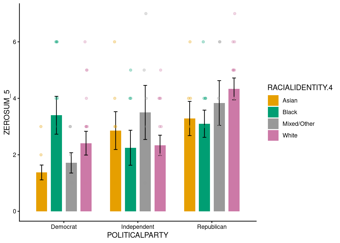
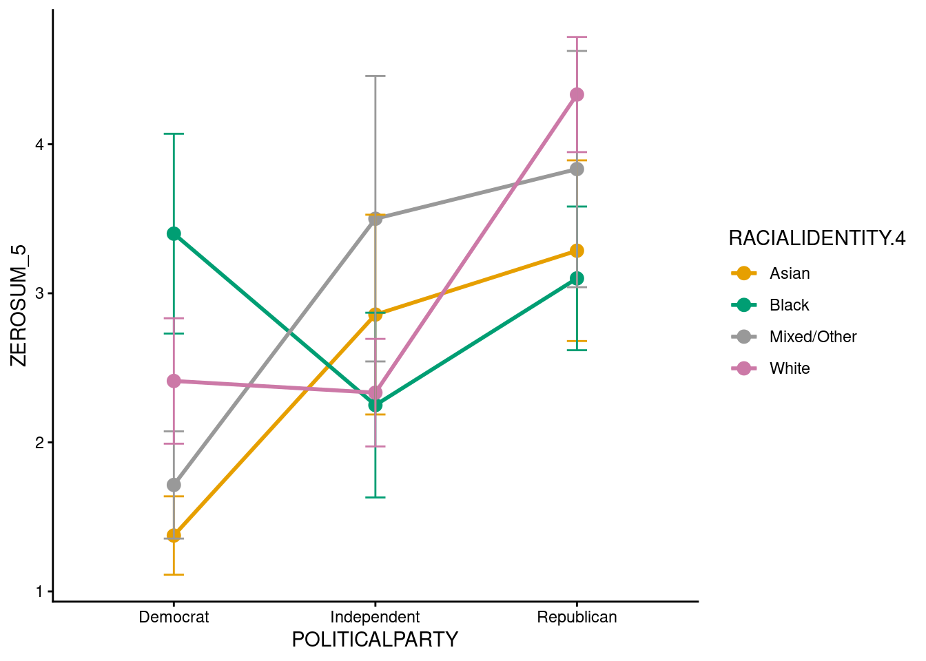
The ANOVA for ZEROSUM_5 indicated a statistically significant main effect of political party, F(2, 104) = 7.98, p < .001. In contrast, the main effect of racial identity and (Racial Identity x Political Party) interaction was not significant.
Warning: Using `size` aesthetic for lines was deprecated in ggplot2 3.4.0.
ℹ Please use `linewidth` instead.
The interaction plot indicated all four racial groups showed a consistent increase in ZEROSUM_5 means moving from Democrat to Independent to Republican. The near significant interaction (p = .052) indicates that these divergent racial group trajectories across party may represent a potential meaningful pattern that warrants replication with a larger sample.
ZEROSUM_6: Gender Based Zero-Sum Beliefs (Gender x Political Party)
In [43]:
Show the code
zerosum6_gender <-aov(ZEROSUM_6 ~ GENDER_cat * POLITICALPARTY, data = select_data)summary(zerosum6_gender)
Df Sum Sq Mean Sq F value Pr(>F)
GENDER_cat 1 0.1 0.05 0.015 0.904
POLITICALPARTY 2 86.3 43.16 12.141 1.74e-05 ***
GENDER_cat:POLITICALPARTY 2 2.4 1.20 0.338 0.714
Residuals 109 387.5 3.55
---
Signif. codes: 0 '***' 0.001 '**' 0.01 '*' 0.05 '.' 0.1 ' ' 1
1 observation deleted due to missingness
The ANOVA for ZEROSUM_6 indicated a statistically significant main effect of political party, F(2, 109) = 12.14, p < .001. In contrast, the main effect of gender and (Gender x Political Party) interaction was not significant.
ZEROSUM_7: More Healthcare for Undocumented Immigrants Means Less for U.S. Citizens (Racial Identity x Political Party)
In [44]:
Show the code
zerosum7_racial <-aov(ZEROSUM_7 ~ RACIALIDENTITY.4* POLITICALPARTY, data = select_data)summary(zerosum7_racial)
Df Sum Sq Mean Sq F value Pr(>F)
RACIALIDENTITY.4 3 9.22 3.072 1.113 0.347621
POLITICALPARTY 2 54.35 27.176 9.842 0.000123 ***
RACIALIDENTITY.4:POLITICALPARTY 6 19.08 3.180 1.152 0.338174
Residuals 102 281.63 2.761
---
Signif. codes: 0 '***' 0.001 '**' 0.01 '*' 0.05 '.' 0.1 ' ' 1
2 observations deleted due to missingness
The ANOVA for ZEROSUM_7 indicated a statistically significant main effect of political party, F(2, 102) = 9.84, p < .001. In contrast, the main effect of racial identity and (Racial Identity x Political Party) interaction was not significant.
ZEROSUM_8: Gender Based Zero-Sum Beliefs (Gender x Political Party)
In [45]:
Show the code
zerosum8_gender <-aov(ZEROSUM_8 ~ GENDER_cat * POLITICALPARTY, data = select_data)summary(zerosum8_gender)
Df Sum Sq Mean Sq F value Pr(>F)
GENDER_cat 1 0.08 0.079 0.033 0.857094
POLITICALPARTY 2 38.85 19.423 8.039 0.000554 ***
GENDER_cat:POLITICALPARTY 2 0.70 0.352 0.145 0.864771
Residuals 109 263.36 2.416
---
Signif. codes: 0 '***' 0.001 '**' 0.01 '*' 0.05 '.' 0.1 ' ' 1
1 observation deleted due to missingness
The ANOVA for ZEROSUM_8 indicated a statistically significant main effect of political party, F(2, 109) = 8.04, p < .001. In contrast, the main effect of gender and (Gender x Political Party) interaction was not significant.
ZEROSUM_9: LGBTQ+ Rights and Religious Freedom (Sexual Identity x Political Party)
In [46]:
Show the code
zerosum9_sexual <-aov(ZEROSUM_9 ~ SEXUAL_IDENTITY_binary * POLITICALPARTY, data = select_data)summary(zerosum9_sexual)
Df Sum Sq Mean Sq F value Pr(>F)
SEXUAL_IDENTITY_binary 1 8.27 8.268 3.263 0.0736 .
POLITICALPARTY 2 61.60 30.798 12.155 1.72e-05 ***
SEXUAL_IDENTITY_binary:POLITICALPARTY 2 4.60 2.301 0.908 0.4063
Residuals 109 276.19 2.534
---
Signif. codes: 0 '***' 0.001 '**' 0.01 '*' 0.05 '.' 0.1 ' ' 1
1 observation deleted due to missingness
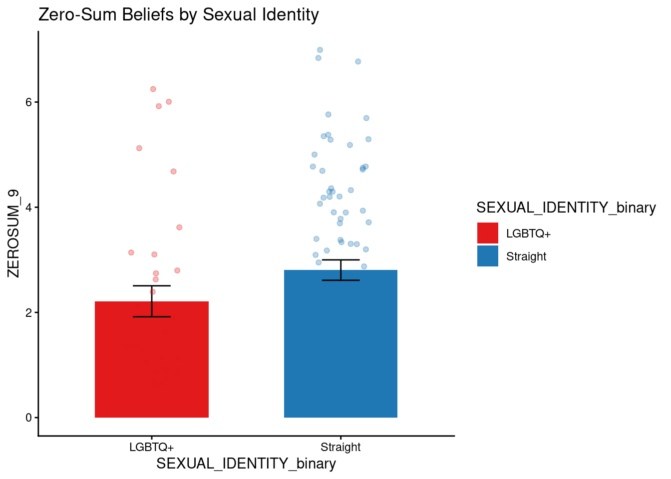
The ANOVA for ZEROSUM_9 indicated a statistically significant main effect of political party, F(2, 109) = 12.16, p < .001. In contrast, the main effect of sexual identity and (Sexual Identity x Political Party) interaction was not significant.
Warning: Removed 1 row containing non-finite outside the scale range (`stat_summary()`).
Removed 1 row containing non-finite outside the scale range (`stat_summary()`).
Warning: Removed 1 row containing missing values or values outside the scale range
(`geom_point()`).
The bar chart for ZEROSUM_9 by sexual identity group revealed that straight identifying respondents endorsed ZEROSUM_9 at a higher mean level relative to LGBTQ+ identifying respondents, a pattern consistent with theoretical expectations.
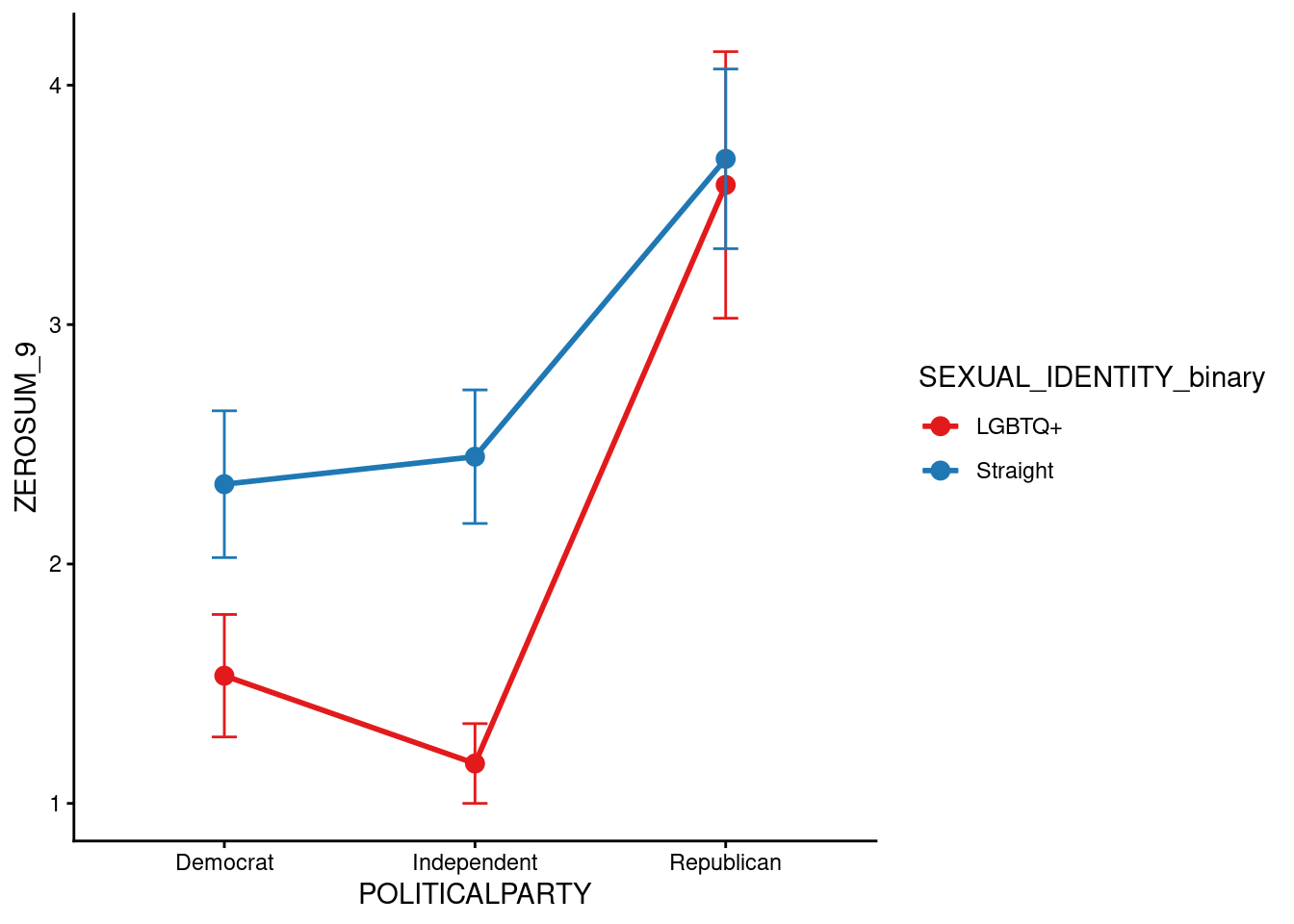
Warning: Removed 1 row containing non-finite outside the scale range (`stat_summary()`).
Removed 1 row containing non-finite outside the scale range (`stat_summary()`).
Removed 1 row containing non-finite outside the scale range (`stat_summary()`).
The interaction plot suggested that this difference between sexual identity groups may have been most pronounced among Republican respondents. However, formal inferential testing of the two-way ANOVA for ZEROSUM_9 did not yield a statistically significant main effect of sexual identity or a significant interaction. The observed visual patterns should therefore be interpreted as descriptive and directional.
ZEROSUM_10: Healthcare Access Zero-Sum Beliefs (Social Status x Political Party)
In [49]:
Show the code
zerosum10_social <-lm(ZEROSUM_10 ~ SOCIALSTATUS * POLITICALPARTY, data = select_data)summary(zerosum10_social)
Call:
lm(formula = ZEROSUM_10 ~ SOCIALSTATUS * POLITICALPARTY, data = select_data)
Residuals:
Min 1Q Median 3Q Max
-3.5768 -1.2394 -0.0234 1.1529 3.3879
Coefficients:
Estimate Std. Error t value Pr(>|t|)
(Intercept) 0.3758 0.8956 0.420 0.67564
SOCIALSTATUS 0.3727 0.1552 2.401 0.01803 *
POLITICALPARTYIndependent 1.4498 1.1639 1.246 0.21556
POLITICALPARTYRepublican 3.2326 1.1977 2.699 0.00805 **
SOCIALSTATUS:POLITICALPARTYIndependent -0.1722 0.2140 -0.805 0.42258
SOCIALSTATUS:POLITICALPARTYRepublican -0.2344 0.2045 -1.146 0.25423
---
Signif. codes: 0 '***' 0.001 '**' 0.01 '*' 0.05 '.' 0.1 ' ' 1
Residual standard error: 1.507 on 110 degrees of freedom
Multiple R-squared: 0.2936, Adjusted R-squared: 0.2615
F-statistic: 9.144 on 5 and 110 DF, p-value: 2.683e-07
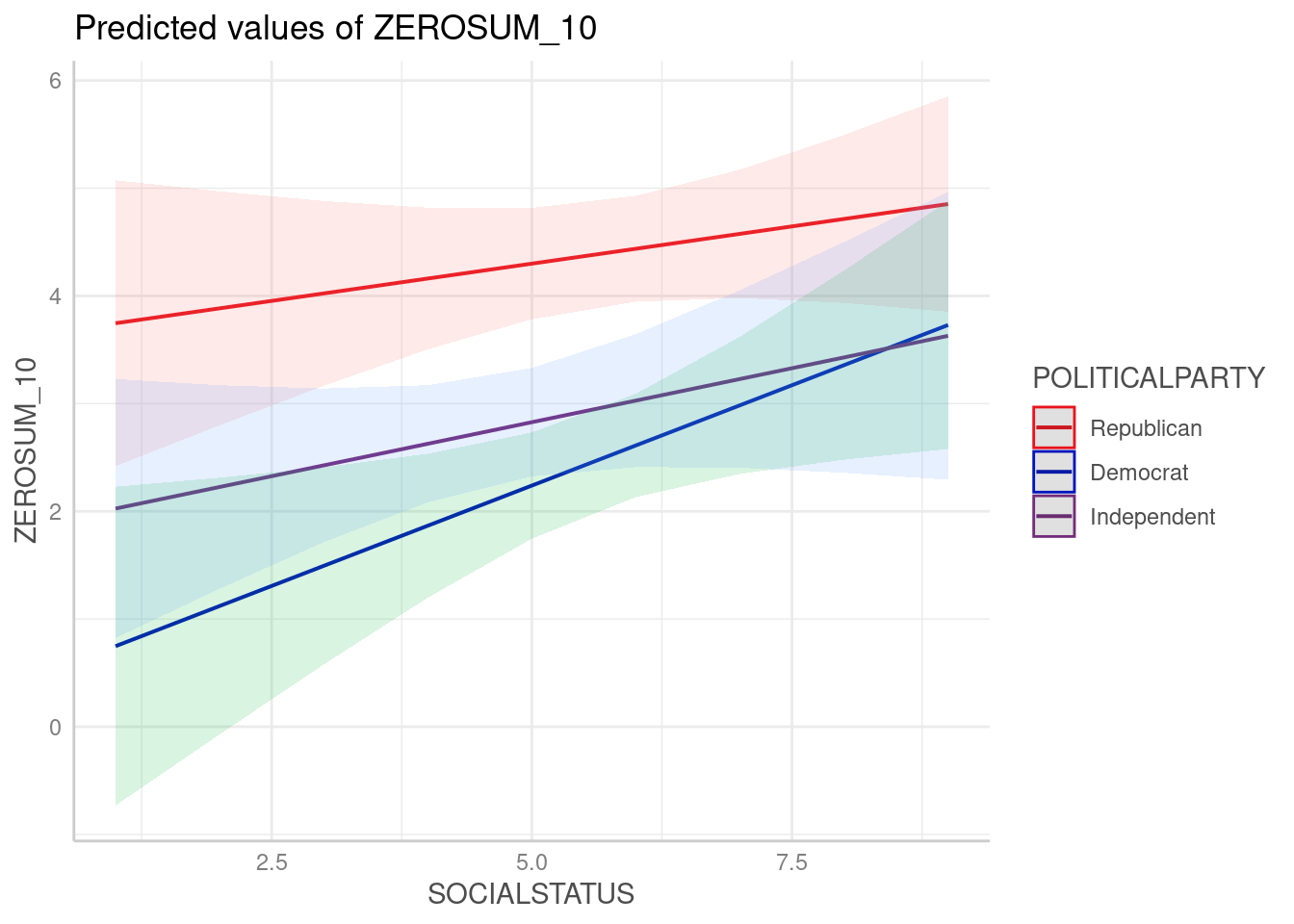
The overall ANCOVA for ZEROSUM_10 model was statistically significant, F(5, 110) = 9.14, p < .001, R-squared = .294, indicating that the model explained approximately 29.4% of the variance in ZEROSUM_10.
For individual predictors, SSS was a significant positive predictor of ZEROSUM_10 (b = 0.37, SE = 0.16, t(110) = 2.40, p = .018), indicating that higher subjective social status was associated with greater endorsement of this healthcare zero-sum belief among Democrats. Among political party, being Republican (vs. Democrat) was associated with significantly higher ZEROSUM_10 at the intercept (b = 3.23, SE = 1.20, t(110) = 2.70, p = .008).
Some of the focal terms are of type `character`. This may lead to
  unexpected results. It is recommended to convert these variables to
  factors before fitting the model.
  The following variables are of type character: `POLITICALPARTY`
Scale for colour is already present.
Adding another scale for colour, which will replace the existing scale.
The predicted marginal means plot suggested that Republicans displayed a uniformly elevated ZEROSUM_10 score across the full range of SSS, while Democrats and Independents showed lower and more overlapping patterns that increased modestly with SSS. Although the interaction terms were not significant, the visual divergence in intercepts reflects the significant main effect of Republican party identification.
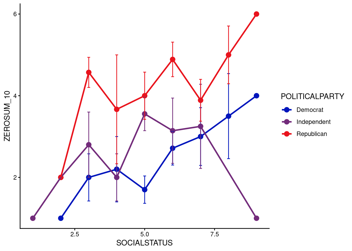
The raw observed data plot similarly shows Republican respondents clustered at higher ZEROSUM_10 values across SSS levels, while Democrats showed a steeper increase from low to high SSS, despite considerable variability.
ZEROSUM_11: Healthcare Access Zero-Sum Beliefs (Income x Political Party)
In [52]:
Show the code
zerosum11_income <-aov(ZEROSUM_11 ~ INCOME * POLITICALPARTY, data = select_data)summary(zerosum11_income)
                      Df Sum Sq Mean Sq F value   Pr(>F)
INCOME                 5   4.74   0.947   0.328 0.895080
POLITICALPARTY         2  50.21  25.103   8.688 0.000338 ***
INCOME:POLITICALPARTY 10   7.18   0.718   0.248 0.990076
Residuals             97 280.28   2.889
---
Signif. codes:  0 '***' 0.001 '**' 0.01 '*' 0.05 '.' 0.1 ' ' 1
1 observation deleted due to missingness
The ANOVA for ZEROSUM_11 indicated a statistically significant main effect of political party, F(2, 97) = 8.69, p < .001. In contrast, the main effect of income and (Income x Political Party) interaction was not significant.