Zero-sum social identity, not zero-sum economic beliefs, explain voting preference in 2024 U.S. presidential election

Introduction

Zero-sum beliefs – the subjective view that as one person gains, others inevitably lose – have been linked to numerous beneficial and harmful social, political, and psychological outcomes (Andrews-Fearon & Davidai (2023)). A zero-sum mindset can be conceptualized as a specific type of competitive belief regarding the relative distribution of limited resources (e.g., physical resources and social status) between two (or more) groups (e.g., racial groups). Although the origin of this mindset can be traced to inter-generational scarcity and high-competition environments for resources, other important factors may partially explain the adoption and centrality of zero-sum beliefs in the current U.S. political discourse.

In a seminal article, Norton & Sommers (2011) demonstrates that White respondents’ perceptions of anti-Black bias has decreased markedly since the 1950s while their perception of anti-White bias has increased significantly during that same period. A decade later, Rasmussen et al. (2022) provide a conceptual replication of these findings and find that “Whites now believe that anti-White bias is more prevalent than anti-Black bias” (p. 1806). The line of research and related studies have led to the modern-day conception of zero-sum racial beliefs, which has been measured frequently using this item: “Less discrimination against minorities means more discrimination against Whites” (Davidai & Ongis (2019)). Chinoy et al. (2023) argue that zero-sum thinking is the root of political differences, demonstrating zero-sum beliefs partially explain a range of social and political views: pro-redistribution policy support, racial attitudes, gender attitudes, and anti-immigration attitudes beyond traditional sociodemographic measures of age, gender, race, income, and state of residence.

Zero-sum racial beliefs are a domain-specific belief about social groups, which differ from zero-sum economic beliefs. For example, people may hold beliefs that policies aimed at reducing income inequality unfairly disadvantage the wealthy, or that initiatives promoting equity give disadvantaged communities an ‘unearned’ advantage over advantaged individuals (Brown et al. (2022)). A plethora of research lines show zero-sum domain-specific beliefs about economic groups and social groups, such as ethnic, citizenship, trade, and income (Chinoy et al. (2023)), as well as perceived competition between immigrants and native-born individuals (Esses et al. (2001)). Though domain-specific beliefs can emerge across many areas, they are often most potent when tied to social identities, when political and interpersonal behavior is strongly influenced by perceived group competition.

Zero-Sum Social Identity Beliefs

Many domain-specific zero-sum beliefs focus on social identity. For example, Wong et al. (2017) found that men with zero-sum gender beliefs have poorer mental health outcomes, worse romantic relationships, and a more polarized view of domestic chores. On the other hand, according to Boland & Davidai (2024), zero-sum political beliefs can lead to a disinterest in political discussion because they lead individuals to antagonize other political ideologies and reduce openness to different ideas, leading to less cross-grup discussion and more polarization. In addition to examining one’s actual standing as a member of a social group, understanding beliefs about one’s own and other social groups may be key for addressing bias and assumptions about resource distribution.

Zero-Sum Economic Beliefs

Zero-sum thinking takes on a unique form when viewed through a more hierarchical lens such as economics. Andrews-Fearon & Davidai (2023) posits that individuals who view the United States as more economically unequal were more likely to hold economic zero-sum beliefs. These individuals were therefore more likely to view the world as unjust. This falls in line with the aforementioned argument that zero-sum ideology often leads to prioritizing dominance and competition. On a more global scale, Hornborg (2003) explains dependency theory, a zero-sum economic framework that acknowledges how certain nations benefit at others expense. This theory claims that some nations exploit the resources of others, leading to the prosperity of the former while the latter suffers. Although economic zero-sum beliefs are much like other types of zero-sum thinking, they differ in that individuals belonging to one’s own group are also thought of as competition. Both on a global and individual scale, the less wealthy are left competing with one another, rather than with the wealthy individuals or groups that oppress them.

Political Party Affiliation

Political party affiliation is a key determinant of voter preference in elections. Several models aim to expain party affiliation and voting based on sociodemographics. For example, Nadeem (2024) found that young people, women, and Black and Hispanic voters tend to be more Democratic leaning. Alternatively, White voters without 4 year degrees tend to lean Republican. However, this methodology struggles in that the social dynamics that determine the relationship between sociodemographics and political affiliation are subject to change. For example, a report by Pew Research Center (2025) examines voting pattern shifts across the 2016, 2020, and 2024 Presidential elections by sociodemographic groups. While some groups tend to be more reliably associated with certain political parties at certain times, these relationships can change meaningfully in a few election cycles. In fact, such drastic shifts have led journalists and academics to speculate on whether a political realignment has taken shape in U.S. politics based on race, class, gender, education and their intersections (Barber & Pope, 2024; Meyer, 2025). However, many prior models have failed to capture the complex arrangements of sociodemographic variables and beliefs influencing voter preference. A (2021) Pew Research Center report provided evidence of 9 different typology groups making up the Republican and Democrat coalitions in 2020. The 6 typology groups within the Republican coalition and 5 typology groups within the Democrat coalition hold very different views on racial bias and social groups, economics, climate change, and health, among others. Prior research demonstrates that zero-sum belief scores differ by political party affiliation, but there is significant variation within political parties (Davis & Sequeira (2024)), suggesting zero-sum beliefs might explain overall differences between parties and identification with specific factions within the Republican and Democrat coalition.

Study Aims

The objective of the study is to: 1) examine domain-specific zero-sum beliefs: zero-sum economic beliefs and zero-sum social identity beliefs, 2) test whether zero-sum beliefs differ based on political party and/or racial identity, 3) test the association between sociodemographic variables and zero-sum beliefs in a logistic regression to explain voter preference for Donald Trump vs. Kamala Harris, and 4) use machine learning models to validate explanatory predict voter preference models.

Methods

Participants and Sampling

More than fifty-five thousand people who are active on the Prolific platform were eligible to complete a 45-minute health beliefs survey with measures on various beliefs associated with politics and health. Using a quota sample by gender (50% Man/ 50% Woman), political affiliation (33% Republican, 33% Democrat, and 34% Independent), and race/RACIALIDENTITY.4 (White 40%, Black 20%, Asian 20%, Mixed 10%, and Other 10%), Prolific recruited one hundred and twenty-five people to complete the survey.

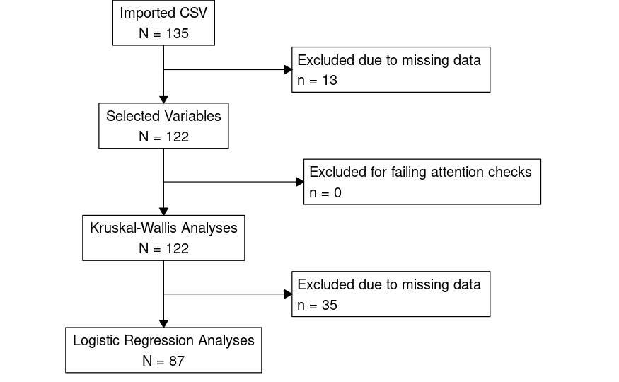
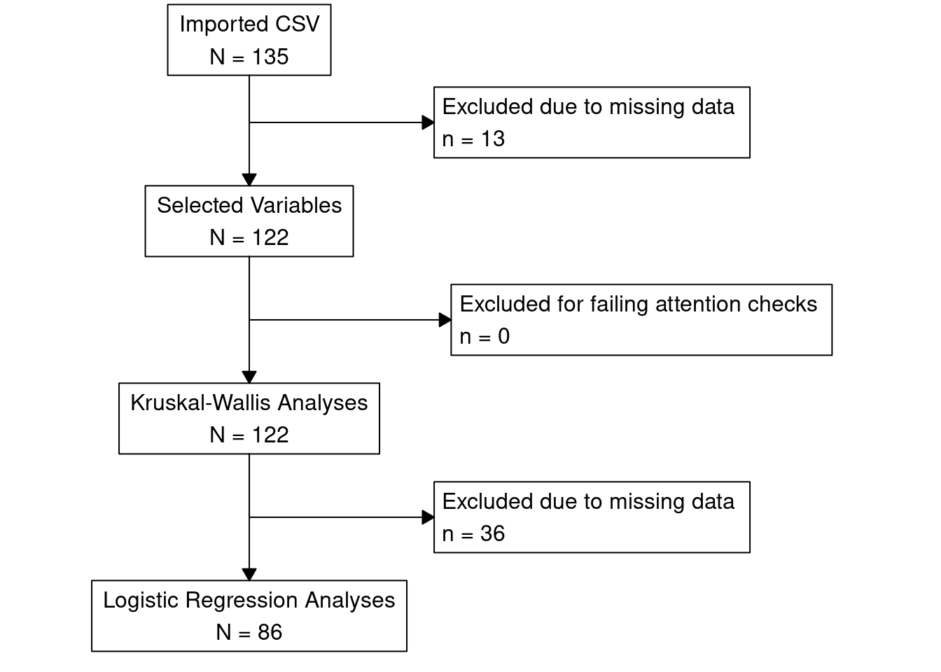
A total of 135 individuals were recruited through Prolific, and 10 were excluded due to incomplete responses, yielding a final analytic sample of 125 participants. The final sample was roughly balanced in terms of gender (50.4% male), racial identity (White: 39.2%, Black: 22.4%, Asian: 18.4%, Mixed/Other: 17.6%), and political affiliation (Democrats: 34.4%, Independents: 32.0%, Republicans: 31.2%).

Figure 1. Participant Flowchart showing exclusions for missing data and final analytic samples used in Kruskal_Wallis and Logistic Regression analyses

Measures

Gender

Respondents reported their gender using the following options: Girl or woman, boy or man, nonbinary/genderfluid/genderqueer, I am not sure/questioning).

Racial Identity

Respondents reported their racial identity using the following options: American Indian or Alaska Native, Asian, Black or African American, Hispanic or Latine, Middle Eastern or North African, Native Hawaiian/Pacific Islander, White, Other).

Subjective Social Status

Respondents reported their subjective social status using MacArthur’s Ladder with the following options Lowest 1 to Highest 10).

Political Beliefs

Respondents reported their political beliefs using the following options: far left/leftist, very liberal, liberal, moderate, conservative, very conservative, alt-right/far-right.

Education

Respondents reported their highest educational attainment using the following options: Some high school or less, High school diploma or GED, Some college, but no degree, Associates or technical degree, Bachelor’s degree, Graduate or professional degree (MA, MS, MBA, PhD, JD, MD, DDS).

Political Party Affiliation

Respondents reported their political party affilaition using the following options: Conservative Party, Democratic Party, Libertarian Party, Republican Party, Socialist or Green Party.

Self-Reported Voting in 2024 U.S. Presidential Election

Respondents reported their voter preference in the 2024 voting behavior using the following selections: Donald Trump, Kamala Harris, Jill Stein, Robert Kennedy Jr., Chase Oliver, Claudia De La Cruz, Cornel West, and DID NOT VOTE IN 2024.

Zero-Sum Beliefs

Respondents were asked to report their level of agreement using a 7-point Likert scale (1: Strongly Disbelieve, 2: Disbelieve, 3: Somewhat Disbelieve, 4: Neither, 5: Somewhat Believe, 6: Believe, 7: Strongly Believe) with .

Respondents were asked to report their level of agreement to 11 zero-sum belief statements using items from two measures and unvalidated, self-generated statements on a 7-point Likert scale (1: Strongly Disbelieve, 2: Disbelieve, 3: Somewhat Disbelieve, 4: Neither Believe Nor Disbelieve, 5: Somewhat Believe, 6: Believe, 7: Strongly Believe). The first three items were selected from the Belief in a Zero Sum Game (BZSG) scale: 1) “Life is so devised that when somebody gains, others have to lose”; 2) “When some people are getting poorer, it means that other people are getting richer”; and 3) “The wealth of a few is acquired at the expense of many” ((Różycka-Tran et al., 2015; Wojciszke et al., 2009)). An additional item was selected from a validated measure capturing beliefs about social identities: 4) “As women face less sexism, men end up facing more sexism” (Wilkins et al. (2015)). Using this sentence construction to examine a gain and loss for two specific groups, seven additional statement were created by the lead author with input from co-authors.

Data Analysis Plan

Data was exported from the qualtrics platform in numerical format and imported into Posit Cloud. R code provided in the data science workflow (Wickham et al. (2016)) was modified to install R packages (see install.R), import data (alldata.csv) using readr, transform sociodemographic variables, such as gender identity (GENDER) to a binary variable (GENDER_MAN) using dplyr, visualize data in a raincloud plot using ggplot2, and model for inferential statistical tests from the stats package along with decision tree and random forest models from the tidymodels package. An exploratory factor analysis using promax rotation was used to examine the factor structure of the eleven items capturing zero sum beliefs.

We analyzed 11 zero-sum belief items (ZEROSUM_), covering both economic and social identity dimensions. Our primary goal was to assess differences across political affiliation (POLITICALPARTY) and racial/ethnic identity (RACIALIDENTITY.4).

First, we conducted a two-way Analysis of Variance (ANOVA) for each zero-sum belief item. To assess whether ANOVA assumptions were met, we used the Shapiro-Wilk test to evaluate the normality of residuals. All 11 items showed non-normality. However, given ANOVA’s robustness to moderate deviations from normality, we further examined residuals using Q-Q plots (qqnorm and qqline) to visualize distributional shape. These plots indicated that the violations were not severe, so we proceeded with ANOVA while noting the assumption limitations.

To address the non-normality more formally and ensure result accuracy, we complemented the ANOVA with a non-parametric Kruskal-Wallis test for each zero-sum belief. This approach allowed us to evaluate group differences without relying on normality assumptions.

Next, an explanatory logistic regression was conducted to classy voter’s preference for Donald Trump (1) vs. Kamala Harris (0) ( TRUMPVOTE ) using POLITICALBELIEFS, ZEROSUM_ECONOMIC, ZEROSUM_IDENTITY, ZEROSUM_1, GENDER_MALE, RELIGIOUS_YES, RACE_BLACK, RACE_ASIAN, RACE_OTHER, EDUCATION_HIGH, and SOCIALSTATUS.

Additionally, we used the tidymodels package in R to classify using a predictive modeling approach. Specifically, both decision tree and random forest classifiers were implemented to predict voter preference.

Using this integrative modeling framework, we provide both explanatory and predictive models for classifying voter preferences.

Results

In [1]:

# Run install.R to ensure packages are installed
source("install.R")

Attaching package: 'dplyr'

The following objects are masked from 'package:stats':

    filter, lag

The following objects are masked from 'package:base':

    intersect, setdiff, setequal, union

Registered S3 methods overwritten by 'ggpp':
  method                  from   
  heightDetails.titleGrob ggplot2
  widthDetails.titleGrob  ggplot2

Attaching package: 'codebook'

The following object is masked from 'package:codebookr':

    codebook

Suggested APA citation: Thériault, R. (2023). rempsyc: Convenience functions for psychology. 
Journal of Open Source Software, 8(87), 5466. https://doi.org/10.21105/joss.05466

Loading required package: carData

Attaching package: 'car'

The following object is masked from 'package:dplyr':

    recode

Attaching package: 'dataMaid'

The following object is masked from 'package:rmarkdown':

    render

The following object is masked from 'package:dplyr':

    summarize

Loading required package: usethis

Attaching package: 'devtools'

The following object is masked from 'package:dataMaid':

    check

Attaching package: 'psych'

The following object is masked from 'package:MBESS':

    cor2cov

The following object is masked from 'package:car':

    logit

The following object is masked from 'package:codebook':

    bfi

The following objects are masked from 'package:ggplot2':

    %+%, alpha

corrplot 0.95 loaded

Loading required package: rpart

randomForest 4.7-1.2

Type rfNews() to see new features/changes/bug fixes.

Attaching package: 'randomForest'

The following object is masked from 'package:psych':

    outlier

The following object is masked from 'package:dplyr':

    combine

The following object is masked from 'package:ggplot2':

    margin

── Attaching packages ────────────────────────────────────── tidymodels 1.3.0 ──

✔ dials        1.4.0     ✔ rsample      1.3.0
✔ infer        1.0.9     ✔ tibble       3.3.0
✔ modeldata    1.4.0     ✔ tune         1.3.0
✔ parsnip      1.3.2     ✔ workflows    1.2.0
✔ purrr        1.1.0     ✔ workflowsets 1.1.1
✔ recipes      1.3.1     ✔ yardstick    1.3.2

── Conflicts ───────────────────────────────────────── tidymodels_conflicts() ──
✖ psych::%+%()            masks ggplot2::%+%()
✖ scales::alpha()         masks psych::alpha(), ggplot2::alpha()
✖ recipes::check()        masks devtools::check(), dataMaid::check()
✖ randomForest::combine() masks dplyr::combine()
✖ purrr::discard()        masks scales::discard()
✖ dplyr::filter()         masks stats::filter()
✖ dplyr::lag()            masks stats::lag()
✖ randomForest::margin()  masks ggplot2::margin()
✖ dials::prune()          masks rpart::prune()
✖ car::recode()           masks dplyr::recode()
✖ purrr::some()           masks car::some()
✖ yardstick::spec()       masks readr::spec()
✖ recipes::step()         masks stats::step()
✖ dataMaid::summarize()   masks dplyr::summarize()
✖ infer::visualize()      masks dataMaid::visualize()

Attaching package: 'kableExtra'

The following object is masked from 'package:dplyr':

    group_rows

Registered S3 method overwritten by 'webshot2':
  method        from   
  print.webshot webshot

Attaching package: 'webshot2'

The following objects are masked from 'package:webshot':

    appshot, resize, rmdshot, shrink, webshot

In [2]:

# Run clean.R to prepare data
source("clean.R")

In [3]:

library(ggplot2)
library(dplyr)
library(tidyr)
library(ggrain)  
library(rmarkdown)
library(readr)
library(patchwork)
library(codebookr)
library(dplyr, warn.conflicts = FALSE)
library(haven)
library(codebook)
library(rempsyc)
library(car)
library(knitr)
library(broom)
library(ggdist)
library(patchwork)
library(car)
library(dataMaid)
library(devtools)
library(MBESS)
library(apaTables)
library(ggpubr)
library(psych)
library(forcats)
library(corrplot)
library(kableExtra)

In [4]:

alldata <- read.csv("data/alldata.csv")

In [5]:

select_data <- read.csv("data/select_data.csv")

In [6]:

#str(select_data)

Descriptive Statistics

In [7]:

# Define Categorical Variables
categorical_vars <- c(
  "EDUCATION_LEVEL", "INCOME", "RELIGIOUS_Identity", "STREETRACE",
  "SEXUAL_IDENTITY", "POLITICALAFFIL", "VOTE_2024", "SERIOUS", "POLITICALPARTY",
  "SEX", "ETHNICITY", "Nationality", "Student.status", "Employment.status",
  "RACIALIDENTITY.6", "RACIALIDENTITY.4"
)

# Define Continuous Variables
continuous_vars <- c(
  "AGE", "SOCIALSTATUS", "POLITICALBELIEFS", "ATTENTION3",
  paste0("ZEROSUM_", 1:11),
  paste0("NEOLIB_", 1:3)
)

In [8]:

library(stringr)

Attaching package: 'stringr'

The following object is masked from 'package:recipes':

    fixed

levels_list <- list(
    EDUCATION_LEVEL = c(
      "Some high school or less",
      "High school diploma or GED",
      "Some college, but no degree",
      "Associates or technical degree",
      "Bachelor’s degree",
      "Graduate or professional degree"
    ),
    ETHNICITY = c(
      "Asian",
      "Black",
      "White",
      "Mixed/Other"
    ),
    Employment.status = c(
      "Part-Time",
      "Full-Time",
      "Unemployed (and job seeking)",
      "Not in paid work (e.g. homemaker', 'retired or disabled)",
      "Due to start a new job within the next month",
      "Other",
      "DATA_EXPIRED"
    ),
    INCOME = c(
      "Less than $25,000",
      "$25,000-$49,999",
      "$50,000-$74,999",
      "$75,000-$99,999",
      "$100,000-$149,999",
      "$150,000 or more",
      "Prefer not to say"
    ),
    Nationality = c(
      "United States"
    ),
    POLITICALAFFIL = c(
      "Conservative Party",
      "Democratic Party",
      "Libertarian Party",
      "Republican Party",
      "Socialist or Green Party",
      "None of the above"
    ),
    POLITICALPARTY = c(
      "Democrat",
      "Republican",
      "Independent"
    ),
    RACIALIDENTITY.4 = c(
      "Asian",
      "Black",
      "White",
      "Mixed/Other"
    ),
    RACIALIDENTITY.6 = c(
      "Asian",
      "Black",
      "White",
      "Latine",
      "Mixed",
      "Other"
    ),
    RELIGIOUS_Identity = c(
      "Christian", "Muslim", "Hindu", "Buddhist", "Jewish", "Folk Religion", "Other", "Religiously Unaffiliated", "Decline to answer"
    ),
    SERIOUS = c("No", "Not Sure", "Yes"),
    SEX = c("Female", "Male"),
    SEXUAL_IDENTITY = c(
      "Straight or heterosexual",
      "Gay or lesbian",
      "Bisexual, pansexual, or queer",
      "Asexual",
      "Not sure"
    ),
    STREETRACE = c(
      "Asian American",
      "Native American/American Indian",
      "White",
      "Latine",
      "Black",
      "Arab",
      "Mexican",
      "Some other race"
    ),
    Student.status = c(
      "Yes",
      "No",
      "DATA_EXPIRED"
    ),
    VOTE_2024 = c(
      "Donald Trump",
      "Kamala Harris",
      "Jill Stein",
      "Robert Kennedy Jr.",
      "Chase Oliver",
      "Claudia De La Cruz",
      "Cornel West",
      "DID NOT VOTE IN 2024"
    )
  )

categorical_table <- select_data %>%
  select(all_of(categorical_vars)) %>%
  pivot_longer(
    cols = everything(),
    names_to = "Variable",
    values_to = "Value"
  ) %>%
  mutate(Value = if_else(is.na(Value), "Missing", Value)) %>%
  group_by(Variable, Value) %>%
  summarise(n = n(), .groups = "drop") %>%
  group_by(Variable) %>%
  mutate(
    percent = paste0(round(100 * n / sum(n), 1), "%"),
    Value = factor(
      Value,
      levels = c(levels_list[[cur_group()$Variable]], "Missing")
    )
  ) %>%
  arrange(Variable, Value) %>%
  ungroup()


kable(
  categorical_table,
  col.names = c("Variable", "Category", "Count", "Percent"),
  caption = "Table 1. Frequencies and Percentages for Categorical Variables",
  booktabs = TRUE,
  row.names = FALSE,
  format = ifelse(knitr::is_latex_output(), "latex", "html")
) %>%
kable_styling(
  latex_options = c("hold_position", "scale_down"),
  bootstrap_options = c("striped", "condensed"),
  full_width = FALSE
  )

Table 1. Frequencies and Percentages for Categorical Variables

Variable	Category	Count	Percent
EDUCATION_LEVEL	High school diploma or GED	7	6%
EDUCATION_LEVEL	Some college, but no degree	19	16.4%
EDUCATION_LEVEL	Associates or technical degree	7	6%
EDUCATION_LEVEL	Bachelor’s degree	45	38.8%
EDUCATION_LEVEL	Graduate or professional degree	38	32.8%
ETHNICITY	Asian	23	19.8%
ETHNICITY	Black	25	21.6%
ETHNICITY	White	45	38.8%
ETHNICITY	Mixed/Other	23	19.8%
Employment.status	Part-Time	28	24.1%
Employment.status	Full-Time	48	41.4%
Employment.status	Unemployed (and job seeking)	10	8.6%
Employment.status	Not in paid work (e.g. homemaker', 'retired or disabled)	10	8.6%
Employment.status	Due to start a new job within the next month	1	0.9%
Employment.status	Other	3	2.6%
Employment.status	DATA_EXPIRED	16	13.8%
INCOME	Less than $25,000	11	9.5%
INCOME	$25,000-$49,999	24	20.7%
INCOME	$50,000-$74,999	21	18.1%
INCOME	$75,000-$99,999	13	11.2%
INCOME	$100,000-$149,999	36	31%
INCOME	$150,000 or more	11	9.5%
Nationality	United States	116	100%
POLITICALAFFIL	Missing	17	14.7%
POLITICALAFFIL	Conservative Party	9	7.8%
POLITICALAFFIL	Democratic Party	49	42.2%
POLITICALAFFIL	Libertarian Party	8	6.9%
POLITICALAFFIL	Republican Party	32	27.6%
POLITICALAFFIL	Socialist or Green Party	1	0.9%
POLITICALPARTY	Democrat	42	36.2%
POLITICALPARTY	Republican	38	32.8%
POLITICALPARTY	Independent	36	31%
RACIALIDENTITY.4	Asian	22	19%
RACIALIDENTITY.4	Black	28	24.1%
RACIALIDENTITY.4	White	47	40.5%
RACIALIDENTITY.4	Mixed/Other	19	16.4%
RACIALIDENTITY.6	Asian	22	19%
RACIALIDENTITY.6	Black	28	24.1%
RACIALIDENTITY.6	White	47	40.5%
RACIALIDENTITY.6	Other	2	1.7%
RACIALIDENTITY.6	Latine	9	7.8%
RACIALIDENTITY.6	Mixed	8	6.9%
RELIGIOUS_Identity	Other	4	3.4%
RELIGIOUS_Identity	Christian	64	55.2%
RELIGIOUS_Identity	Muslim	2	1.7%
RELIGIOUS_Identity	Hindu	2	1.7%
RELIGIOUS_Identity	Jewish	1	0.9%
RELIGIOUS_Identity	Religiously Unaffiliated	40	34.5%
RELIGIOUS_Identity	Decline to answer	3	2.6%
SERIOUS	Missing	1	0.9%
SERIOUS	Yes	115	99.1%
SEX	Female	57	49.1%
SEX	Male	59	50.9%
SEXUAL_IDENTITY	Straight or heterosexual	83	71.6%
SEXUAL_IDENTITY	Gay or lesbian	10	8.6%
SEXUAL_IDENTITY	Bisexual, pansexual, or queer	21	18.1%
SEXUAL_IDENTITY	Asexual	2	1.7%
STREETRACE	Missing	1	0.9%
STREETRACE	Black	30	25.9%
STREETRACE	White	51	44%
STREETRACE	Latine	7	6%
STREETRACE	Asian American	21	18.1%
STREETRACE	Native American/American Indian	3	2.6%
STREETRACE	Mexican	3	2.6%
Student.status	DATA_EXPIRED	18	15.5%
Student.status	No	70	60.3%
Student.status	Yes	28	24.1%
VOTE_2024	Missing	3	2.6%
VOTE_2024	Donald Trump	50	43.1%
VOTE_2024	Kamala Harris	46	39.7%
VOTE_2024	Chase Oliver	1	0.9%
VOTE_2024	Cornel West	1	0.9%
VOTE_2024	DID NOT VOTE IN 2024	15	12.9%

In [9]:

desc_table_continuous <- select_data %>%
  select(all_of(continuous_vars)) %>%
  psych::describe() %>%
  tibble::rownames_to_column(var = "Variable") %>%
  select(Variable, n, mean, median, sd, min, max)

if (knitr::is_html_output()) {
  knitr::kable(
    desc_table_continuous,
    digits = 2,
    escape = TRUE,
    format = "html",
    caption = "Table 2. Descriptive Statistics Table for Continuous Variables"
  ) %>%
    kableExtra::kable_styling(bootstrap_options = c("striped", "hover", "condensed"))
} else if (knitr::is_latex_output()) {
  knitr::kable(
    desc_table_continuous,
    digits = 2,
    escape = TRUE,
    format = "latex",
    longtable = TRUE,
    caption = "Descriptive Statistics Table for Continuous Variables"
  ) %>%
    kableExtra::kable_styling(latex_options = "scale_down")
}

Table 2. Descriptive Statistics Table for Continuous Variables

Variable	n	mean	median	sd	min	max
AGE	115	36.21	33	12.88	19	73
SOCIALSTATUS	116	5.35	6	1.74	1	9
POLITICALBELIEFS	114	3.68	4	1.35	1	6
ATTENTION3	116	2.00	2	0.00	2	2
ZEROSUM_1	116	3.93	4	1.73	1	7
ZEROSUM_2	115	4.73	5	1.61	1	7
ZEROSUM_3	115	4.89	5	1.50	1	7
ZEROSUM_4	115	3.05	3	1.63	1	6
ZEROSUM_5	116	2.88	3	1.77	1	7
ZEROSUM_6	115	3.43	3	2.04	1	7
ZEROSUM_7	114	3.54	4	1.80	1	7
ZEROSUM_8	115	2.99	3	1.63	1	7
ZEROSUM_9	115	2.63	2	1.75	1	7
ZEROSUM_10	116	3.19	3	1.75	1	7
ZEROSUM_11	115	3.20	3	1.73	1	7
NEOLIB_1	113	4.85	5	1.05	2	6
NEOLIB_2	115	4.37	5	1.34	1	6
NEOLIB_3	110	4.15	4	1.42	1	6

Table 2 reports the descriptive statistics (count, mean, median, sd, min, max) for all study variables. The sample consisted of 116 participants, with a mean age of 36.21 years (SD = 12.88, range = 19–73). Participants reported a mean social status of 5.35 (SD = 1.74) on a 10-point scale.

Zero-sum belief items were rated on a 7-point scale with neutral in the middle. For Item 1, the average score was close to neutral (M = 3.92). Items 2 and 3 had higher average scores (M = 4.75 and M = 4.92, respectively), indicating general agreement. Items 4 through 11 showed lower average scores (ranging from 2.59 to 3.52), reflecting more disagreement than agreement with those statements.

In [10]:

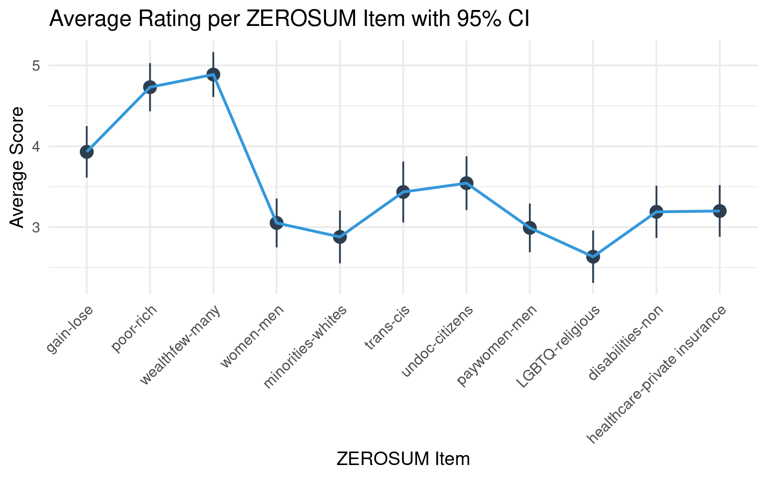
# select and reshape the ZEROSUM items
zerosum_long <- select_data %>%
  select(starts_with("ZEROSUM_")) %>%
  pivot_longer(
    cols = everything(),
    names_to = "Item",
    values_to = "Score"
  )

# mean score per item
zerosum_summary <- zerosum_long %>%
  group_by(Item) %>%
  summarise(
    MeanScore = mean(Score, na.rm = TRUE),
    n = sum(!is.na(Score)),
    sd = sd(Score, na.rm = TRUE),
    se = sd / sqrt(n),                           
    CI_lower = MeanScore - qt(0.975, n - 1) * se, # Lower 95% CI
    CI_upper = MeanScore + qt(0.975, n - 1) * se, # Upper 95% CI
    .groups = "drop"
  ) %>%
  mutate(Item = factor(Item, levels = paste0("ZEROSUM_", 1:11)))


item_labels <- c(
  "gain-lose",
  "poor-rich",
  "wealthfew-many",
  "women-men",
  "minorities-whites",
  "trans-cis",
  "undoc-citizens",
  "paywomen-men",
  "LGBTQ-religious",
  "disabilities-non",
  "healthcare-private insurance"
)


ggplot(zerosum_summary, aes(x = Item, y = MeanScore)) +
  geom_pointrange(aes(ymin = CI_lower, ymax = CI_upper),
                  color = "#2c3e50", size = 0.8) +
  geom_line(aes(group = 1), color = "#3498db", linewidth = 1) +
  theme_minimal(base_size = 14) +
  scale_x_discrete(labels = item_labels) +
  labs(
    title = "Average Rating per ZEROSUM Item with 95% CI",
    x = "ZEROSUM Item",
    y = "Average Score"
  ) +
  theme(axis.text.x = element_text(angle = 45, hjust = 1))

Average ratings for each ZEROSUM item with 95% confidence intervals. Items 2 (“poor-rich”) and 3 (“wealthfew-many”) received the highest ratings. Item 1 (“gain-lose”) was rated moderately, while items 4 through 11 had the lowest average ratings.

Factor Analysis

Factor Analysis of Zero-Sum Beliefs

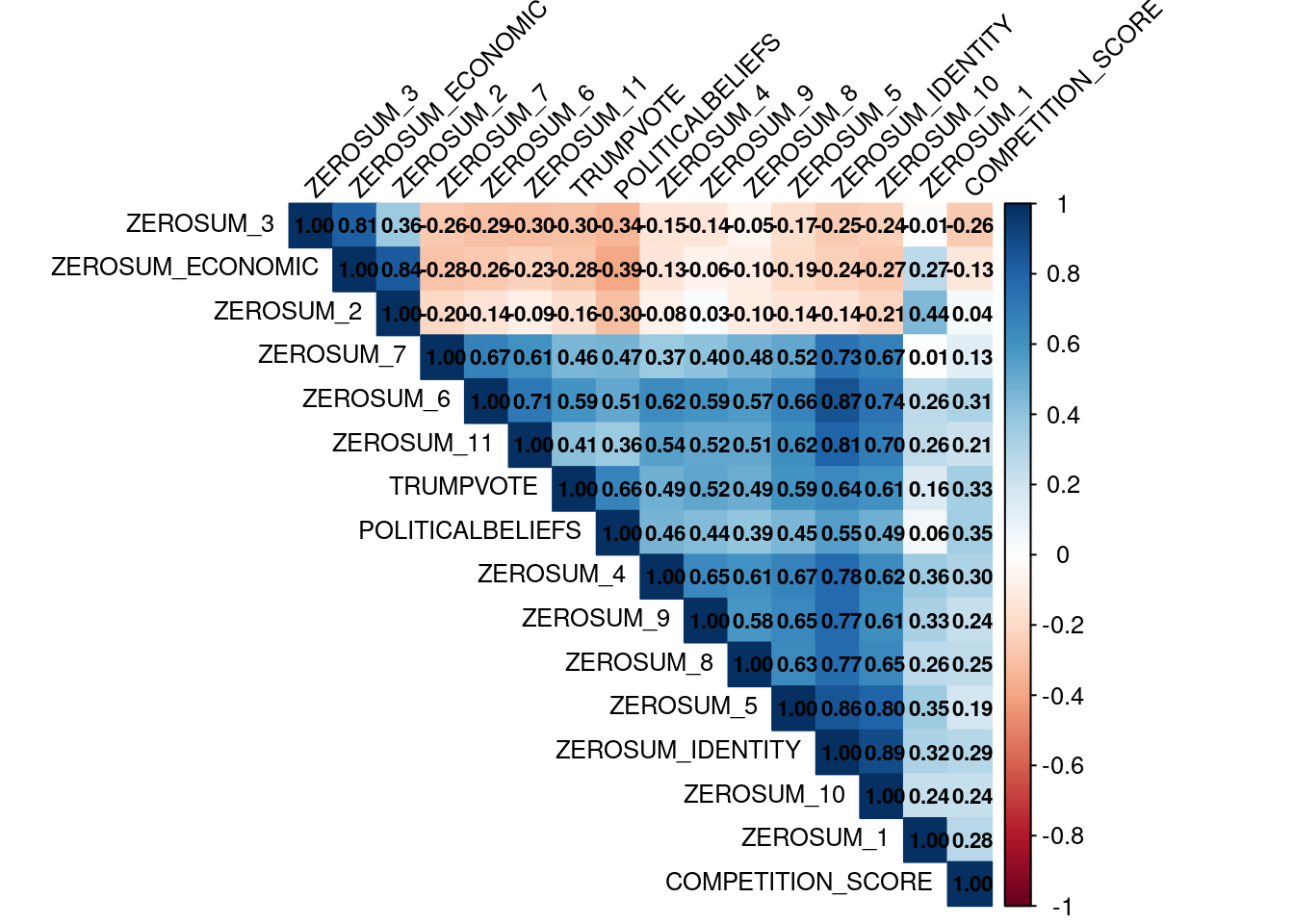
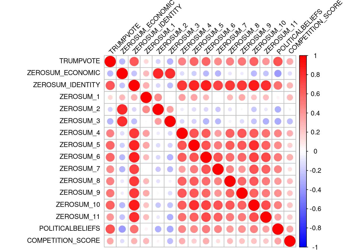
The output below displays the correlation matrix of the Zero-Sum Beliefs items. Each cell represents the Pearson correlation between pairs of items. ZEROSUM_1 is moderately positively correlated with most of the other zero-sum items (r = .092 - .462), suggesting a general zero-sum thinking. ZEROSUM_2 and ZEROSUM_3 also show a moderate positive correlation with each other (r = .479). Most notably, ZEROSUM_4 through ZEROSUM_11 are consistently and positively correlated, with moderately positive correlations (ranging from 0.46 to 0.68), indicating a strong internal consistency among these items. This pattern supports the idea that these items are likely capturing a common latent construct.

In [11]:

library(psych)
# create data frame of ZEROSUM variables for factor analysis
df.ZEROSUM <- select_data[, c("ZEROSUM_1", "ZEROSUM_2", "ZEROSUM_3", "ZEROSUM_4", 
                                  "ZEROSUM_5", "ZEROSUM_6", "ZEROSUM_7", "ZEROSUM_8", 
                                  "ZEROSUM_9", "ZEROSUM_10", "ZEROSUM_11")]

# Or using dplyr to select variables
# zerosum_vars <- select_data %>% select(ZEROSUM_1:ZEROSUM_11)

# Check the correlation matrix first
cor_matrix <- cor(df.ZEROSUM, use = "complete.obs")

kable(
  round(cor_matrix, 2),
  caption = "Table 27. Correlation Matrix of Zero-Sum Belief Items",
  booktabs = TRUE
) %>%
  kable_styling(
    latex_options = c("hold_position", "scale_down"),
    full_width = FALSE
  )

Table 27. Correlation Matrix of Zero-Sum Belief Items

	ZEROSUM_1	ZEROSUM_2	ZEROSUM_3	ZEROSUM_4	ZEROSUM_5	ZEROSUM_6	ZEROSUM_7	ZEROSUM_8	ZEROSUM_9	ZEROSUM_10	ZEROSUM_11
ZEROSUM_1	1.00	0.38	0.08	0.40	0.34	0.31	0.08	0.23	0.40	0.26	0.24
ZEROSUM_2	0.38	1.00	0.47	-0.02	-0.01	0.01	-0.09	-0.16	0.08	-0.12	-0.04
ZEROSUM_3	0.08	0.47	1.00	-0.06	-0.11	-0.19	-0.14	-0.13	-0.11	-0.20	-0.21
ZEROSUM_4	0.40	-0.02	-0.06	1.00	0.63	0.57	0.33	0.51	0.57	0.48	0.45
ZEROSUM_5	0.34	-0.01	-0.11	0.63	1.00	0.61	0.54	0.58	0.62	0.69	0.57
ZEROSUM_6	0.31	0.01	-0.19	0.57	0.61	1.00	0.55	0.50	0.59	0.68	0.68
ZEROSUM_7	0.08	-0.09	-0.14	0.33	0.54	0.55	1.00	0.42	0.37	0.60	0.55
ZEROSUM_8	0.23	-0.16	-0.13	0.51	0.58	0.50	0.42	1.00	0.51	0.58	0.49
ZEROSUM_9	0.40	0.08	-0.11	0.57	0.62	0.59	0.37	0.51	1.00	0.60	0.53
ZEROSUM_10	0.26	-0.12	-0.20	0.48	0.69	0.68	0.60	0.58	0.60	1.00	0.70
ZEROSUM_11	0.24	-0.04	-0.21	0.45	0.57	0.68	0.55	0.49	0.53	0.70	1.00

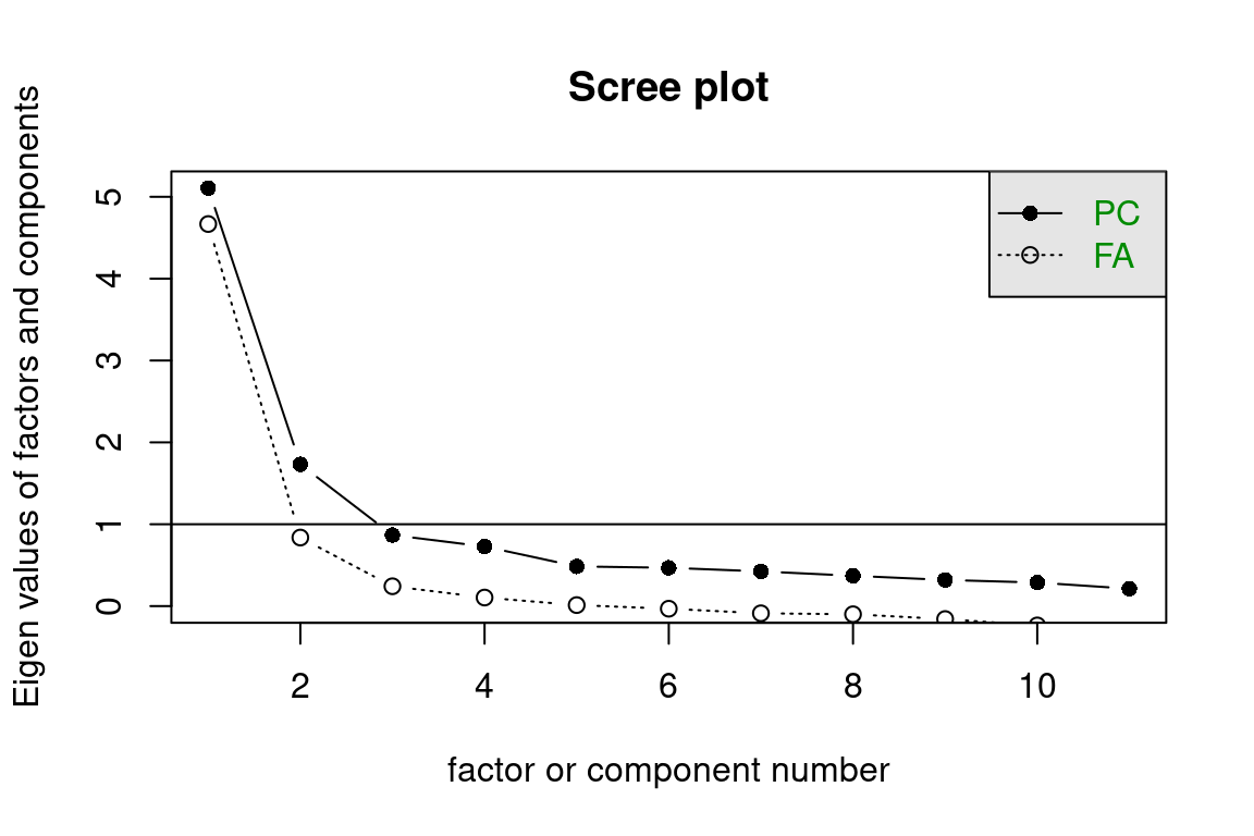
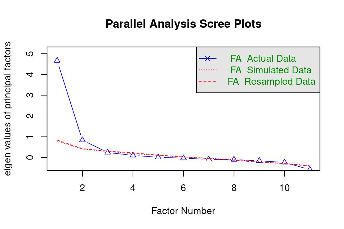
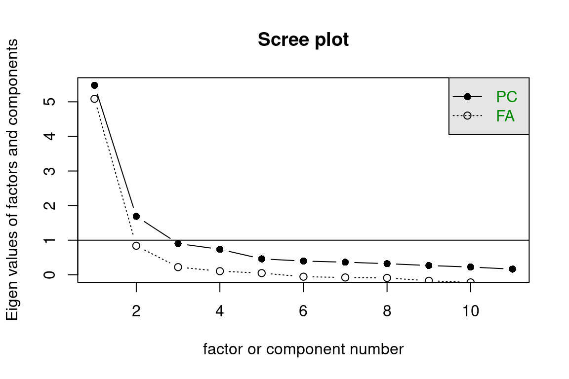
# Determine number of factors using scree plot and parallel analysis
scree(df.ZEROSUM)

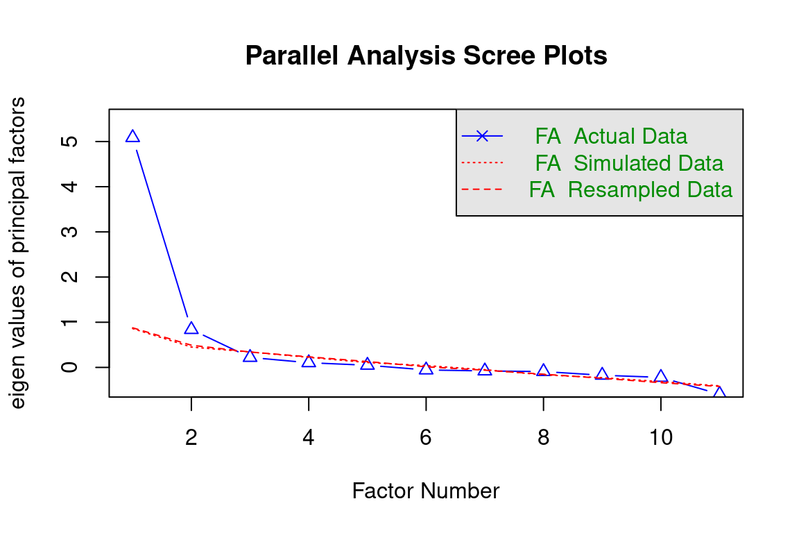
wrapped_fa_parallel <- paste(strwrap(capture.output(fa.parallel(df.ZEROSUM, fa = "fa")), width = 80), collapse = "\n")

cat(wrapped_fa_parallel, "\n")

Parallel analysis suggests that the number of factors = 2 and the number of
components = NA 

# Run 2-factor factor analysis (adjust nfactors based on scree plot/parallel analysis)
fa_result <- fa(df.ZEROSUM, 
                nfactors = 2,  # adjust this number based on your analysis
                rotate = "promax",
                fm = "ml")  # maximum likelihood

Loading required namespace: GPArotation

# View results
print(fa_result)

Factor Analysis using method =  ml
Call: fa(r = df.ZEROSUM, nfactors = 2, rotate = "promax", fm = "ml")
Standardized loadings (pattern matrix) based upon correlation matrix
             ML2   ML1   h2    u2 com
ZEROSUM_1   0.41  0.39 0.31 0.688 2.0
ZEROSUM_2   0.00  1.00 1.00 0.005 1.0
ZEROSUM_3  -0.18  0.47 0.26 0.742 1.3
ZEROSUM_4   0.67  0.00 0.45 0.546 1.0
ZEROSUM_5   0.81  0.01 0.66 0.337 1.0
ZEROSUM_6   0.81  0.03 0.65 0.348 1.0
ZEROSUM_7   0.64 -0.08 0.42 0.583 1.0
ZEROSUM_8   0.67 -0.15 0.47 0.528 1.1
ZEROSUM_9   0.74  0.10 0.55 0.445 1.0
ZEROSUM_10  0.84 -0.11 0.73 0.271 1.0
ZEROSUM_11  0.77 -0.03 0.59 0.406 1.0

                       ML2  ML1
SS loadings           4.67 1.43
Proportion Var        0.42 0.13
Cumulative Var        0.42 0.55
Proportion Explained  0.77 0.23
Cumulative Proportion 0.77 1.00

 With factor correlations of 
      ML2   ML1
ML2  1.00 -0.02
ML1 -0.02  1.00

Mean item complexity =  1.1
Test of the hypothesis that 2 factors are sufficient.

df null model =  55  with the objective function =  5.55 with Chi Square =  613.32
df of  the model are 34  and the objective function was  0.49 

The root mean square of the residuals (RMSR) is  0.05 
The df corrected root mean square of the residuals is  0.06 

The harmonic n.obs is  115 with the empirical chi square  31.85  with prob <  0.57 
The total n.obs was  116  with Likelihood Chi Square =  53.46  with prob <  0.018 

Tucker Lewis Index of factoring reliability =  0.943
RMSEA index =  0.07  and the 90 % confidence intervals are  0.03 0.105
BIC =  -108.16
Fit based upon off diagonal values = 0.99
Measures of factor score adequacy             
                                                   ML2  ML1
Correlation of (regression) scores with factors   0.96 1.00
Multiple R square of scores with factors          0.92 1.00
Minimum correlation of possible factor scores     0.84 0.99

fa_result$loadings

Loadings:
           ML2    ML1   
ZEROSUM_1   0.405  0.394
ZEROSUM_2          0.998
ZEROSUM_3  -0.176  0.473
ZEROSUM_4   0.674       
ZEROSUM_5   0.814       
ZEROSUM_6   0.808       
ZEROSUM_7   0.639       
ZEROSUM_8   0.668 -0.148
ZEROSUM_9   0.740       
ZEROSUM_10  0.845 -0.106
ZEROSUM_11  0.769       

                 ML2   ML1
SS loadings    4.672 1.425
Proportion Var 0.425 0.130
Cumulative Var 0.425 0.554

# Get factor scores
factor_scores <- fa_result$scores

The results of the factor analysis – an unsupervised machine learning technique – support a two factor model with a promax rotation. The first item loads equally on each factor and will not be included in the composite construction. Based on the items, we named the first factor as ZEROSUM_ECONOMIC and the second factor as ZEROSUM_IDENTITY to correspond with the two different referents of economic (e.g., wealth vs. poor) and social identity (e.g., racial minorities vs. white people), respectively. The IDENTITY factor showed high reliability, with a Cronbach’s alpha of 0.91. This means the items in the ZEROSUM_IDENTITY scale consistently measure the same social identity concept.

In [12]:

select_data <- select_data %>%
  mutate(
    ZEROSUM_ECONOMIC = (ZEROSUM_2 + ZEROSUM_3)/2,
    ZEROSUM_IDENTITY = (ZEROSUM_4 + ZEROSUM_5 + ZEROSUM_6 + ZEROSUM_7 + ZEROSUM_8 + ZEROSUM_9 + ZEROSUM_10 + ZEROSUM_11)/8
  )

Reliability of Zero Sum Social Identity Beliefs

library(psych)
library(knitr)

alpha_identity <- psych::alpha(
  select_data[, c(
    "ZEROSUM_4", "ZEROSUM_5", "ZEROSUM_6",
    "ZEROSUM_7", "ZEROSUM_8", "ZEROSUM_9",
    "ZEROSUM_10", "ZEROSUM_11"
  )]
)

kable(
    as.data.frame(alpha_identity$total),
    caption = "Table 4. Overall Reliability Statistics (Cronbach’s Alpha)",
    digits = 3
)

Table 4. Overall Reliability Statistics (Cronbach’s Alpha)

	raw_alpha	std.alpha	G6(smc)	average_r	S/N	ase	mean	sd	median_r
	0.909	0.909	0.908	0.554	9.942	0.013	3.102	1.388	0.568

ci_df <- data.frame(
  Method = "Feldt",
  Lower = alpha_identity$feldt$lower.ci$raw_alpha,
  Alpha = alpha_identity$feldt$alpha$raw_alpha,
  Upper = alpha_identity$feldt$upper.ci$raw_alpha
)

kable(
  ci_df,
  caption = "Table 5. 95% confidence boundaries",
  digits = 2,
  booktabs = TRUE
)

Table 5. 95% confidence boundaries

Method	Lower	Alpha	Upper
Feldt	0.88	0.91	0.93

kable(
    alpha_identity$alpha.drop,
    caption = "Table 6. Reliability if an item is dropped",
    digits = 2
)

Table 6. Reliability if an item is dropped

	raw_alpha	std.alpha	G6(smc)	average_r	S/N	alpha se	var.r	med.r
ZEROSUM_4	0.90	0.90	0.90	0.57	9.28	0.01	0.01	0.58
ZEROSUM_5	0.89	0.89	0.89	0.54	8.11	0.02	0.01	0.55
ZEROSUM_6	0.89	0.89	0.89	0.54	8.22	0.02	0.01	0.55
ZEROSUM_7	0.91	0.91	0.90	0.58	9.60	0.01	0.01	0.58
ZEROSUM_8	0.90	0.90	0.90	0.57	9.21	0.01	0.01	0.57
ZEROSUM_9	0.90	0.90	0.90	0.56	8.83	0.01	0.01	0.57
ZEROSUM_10	0.89	0.89	0.88	0.53	7.97	0.02	0.01	0.55
ZEROSUM_11	0.89	0.90	0.89	0.55	8.54	0.01	0.01	0.57

kable(
    alpha_identity$item.stats,
    caption = "Table 7. Item Statistics",
    digits = 2
)

Table 7. Item Statistics

	n	raw.r	std.r	r.cor	r.drop	mean	sd
ZEROSUM_4	115	0.72	0.73	0.68	0.64	3.05	1.63
ZEROSUM_5	116	0.84	0.84	0.82	0.78	2.88	1.77
ZEROSUM_6	115	0.84	0.83	0.81	0.77	3.43	2.04
ZEROSUM_7	114	0.70	0.70	0.64	0.61	3.54	1.80
ZEROSUM_8	115	0.73	0.73	0.67	0.64	2.99	1.63
ZEROSUM_9	115	0.77	0.77	0.73	0.69	2.63	1.75
ZEROSUM_10	116	0.86	0.85	0.84	0.80	3.19	1.75
ZEROSUM_11	115	0.80	0.80	0.77	0.73	3.20	1.73

kable(as.data.frame.matrix(alpha_identity$response.freq),
      digits = 2,
      caption = "Table 8. Non missing response frequency for each item")

Table 8. Non missing response frequency for each item

	1	2	3	4	5	6	7	miss
ZEROSUM_4	0.28	0.10	0.19	0.21	0.15	0.07	0.00	0.01
ZEROSUM_5	0.36	0.08	0.20	0.17	0.08	0.09	0.02	0.00
ZEROSUM_6	0.30	0.09	0.13	0.14	0.14	0.14	0.07	0.01
ZEROSUM_7	0.21	0.11	0.11	0.23	0.23	0.06	0.05	0.02
ZEROSUM_8	0.30	0.09	0.21	0.22	0.14	0.03	0.02	0.01
ZEROSUM_9	0.42	0.12	0.15	0.13	0.11	0.04	0.03	0.01
ZEROSUM_10	0.28	0.09	0.19	0.16	0.16	0.10	0.01	0.00
ZEROSUM_11	0.24	0.15	0.15	0.23	0.11	0.10	0.02	0.01

Reliability of Zero Sum Economic Beliefs

In [13]:

library(psych)

# Alpha for ZEROSUM_ECONOMIC (2 items)
alpha_economic <- psych::alpha(select_data[, c("ZEROSUM_2", "ZEROSUM_3")])

kable(
    as.data.frame(alpha_economic$total),
    caption = "Table 9. Overall Reliability Statistics (Cronbach’s Alpha)",
    digits = 3
)

Table 9. Overall Reliability Statistics (Cronbach’s Alpha)

	raw_alpha	std.alpha	G6(smc)	average_r	S/N	ase	mean	sd	median_r
	0.644	0.645	0.476	0.476	1.815	0.066	4.809	1.339	0.476

ci_df_eco <- data.frame(
  Method = "Feldt",
  Lower = alpha_economic$feldt$lower.ci$raw_alpha,
  Alpha = alpha_economic$feldt$alpha$raw_alpha,
  Upper = alpha_economic$feldt$upper.ci$raw_alpha
)

kable(
  ci_df_eco,
  caption = "Table 10. 95% confidence boundaries",
  digits = 2,
  booktabs = TRUE
)

Table 10. 95% confidence boundaries

Method	Lower	Alpha	Upper
Feldt	0.49	0.64	0.75

kable(
    alpha_economic$alpha.drop,
    caption = "Table 11. Reliability if an item is dropped",
    digits = 2
)

Table 11. Reliability if an item is dropped

	raw_alpha	std.alpha	G6(smc)	average_r	S/N	alpha se	var.r	med.r
ZEROSUM_2	0.51	0.48	0.23	0.48	0.91	NA	0	0.48
ZEROSUM_3	0.44	0.48	0.23	0.48	0.91	NA	0	0.48

kable(
    alpha_economic$item.stats,
    caption = "Table 12. Item Statistics",
    digits = 2
)

Table 12. Item Statistics

	n	raw.r	std.r	r.cor	r.drop	mean	sd
ZEROSUM_2	115	0.87	0.86	0.59	0.48	4.73	1.61
ZEROSUM_3	115	0.85	0.86	0.59	0.48	4.89	1.50

kable(as.data.frame.matrix(alpha_economic$response.freq),
      digits = 2,
      caption = "Table 13. Non missing response frequency for each item")

Table 13. Non missing response frequency for each item

	1	2	3	4	5	6	7	miss
ZEROSUM_2	0.04	0.06	0.10	0.21	0.27	0.16	0.17	0.01
ZEROSUM_3	0.03	0.06	0.06	0.22	0.28	0.20	0.16	0.01

The zero-sum economic beliefs factor showed lower reliability, with a Cronbach’s alpha of 0.65. A lower reliability is expected in a two-item measure.

Factor Analysis of Neoliberal Mindset

In [14]:

library(psych)

# create data frame of NEOLIB variables
df.NEOLIB <- select_data[, c("NEOLIB_1", "NEOLIB_2", "NEOLIB_3")]

# correlation matrix
cor_matrix_neolib <- cor(df.NEOLIB, use = "complete.obs")
kable(
  round(cor_matrix_neolib, 3),
  caption = "Table 14. Correlation Matrix for NEOLIB Scale",
  booktabs = TRUE
)

Table 14. Correlation Matrix for NEOLIB Scale

	NEOLIB_1	NEOLIB_2	NEOLIB_3
NEOLIB_1	1.000	0.380	0.422
NEOLIB_2	0.380	1.000	0.638
NEOLIB_3	0.422	0.638	1.000

# Cronbach’s alpha for internal consistency
alpha_neolib <- psych::alpha(df.NEOLIB)

kable(
    as.data.frame(alpha_neolib$total),
    caption = "Table 15. Overall Reliability Statistics (Cronbach’s Alpha)",
    digits = 3
)

Table 15. Overall Reliability Statistics (Cronbach’s Alpha)

	raw_alpha	std.alpha	G6(smc)	average_r	S/N	ase	mean	sd	median_r
	0.74	0.739	0.676	0.486	2.835	0.04	4.466	1.065	0.422

ci_df_neo <- data.frame(
  Method = "Feldt",
  Lower = alpha_neolib$feldt$lower.ci$raw_alpha,
  Alpha = alpha_neolib$feldt$alpha$raw_alpha,
  Upper = alpha_neolib$feldt$upper.ci$raw_alpha,
  r_bar = alpha_neolib$feldt$r.bar$raw_alpha
)

kable(
  ci_df_neo,
  caption = "Table 16. 95% confidence boundaries",
  digits = 2,
  booktabs = TRUE
)

Table 16. 95% confidence boundaries

Method	Lower	Alpha	Upper	r_bar
Feldt	0.65	0.74	0.81	0.49

kable(
    alpha_neolib$alpha.drop,
    caption = "Table 17. Reliability if an item is dropped",
    digits = 2
)

Table 17. Reliability if an item is dropped

	raw_alpha	std.alpha	G6(smc)	average_r	S/N	alpha se	var.r	med.r
NEOLIB_1	0.78	0.78	0.64	0.64	3.62	0.04	NA	0.64
NEOLIB_2	0.57	0.59	0.42	0.42	1.46	0.08	NA	0.42
NEOLIB_3	0.55	0.56	0.39	0.39	1.29	0.08	NA	0.39

kable(
    alpha_neolib$item.stats,
    caption = "Table 18. Item Statistics",
    digits = 2
)

Table 18. Item Statistics

	n	raw.r	std.r	r.cor	r.drop	mean	sd
NEOLIB_1	113	0.71	0.75	0.51	0.45	4.85	1.05
NEOLIB_2	115	0.85	0.84	0.73	0.63	4.37	1.34
NEOLIB_3	110	0.88	0.85	0.76	0.65	4.15	1.42

kable(as.data.frame.matrix(alpha_neolib$response.freq),
      digits = 2,
      caption = "Table 19. Non missing response frequency for each item")

Table 19. Non missing response frequency for each item

	1	2	3	4	5	6	miss
NEOLIB_1	0.00	0.04	0.06	0.24	0.35	0.32	0.03
NEOLIB_2	0.03	0.08	0.15	0.23	0.29	0.23	0.01
NEOLIB_3	0.06	0.08	0.14	0.25	0.30	0.17	0.05

# factor analysis (1 factor)
fa_neolib <- fa(df.NEOLIB,
                nfactors = 1,
                rotate = "none",
                fm = "ml")

kable(
  round(fa_neolib$loadings[1:3, 1, drop = FALSE], 3),
  caption = "Table 20. Factor Loadings for NEOLIB Scale",
  booktabs = TRUE
)

Table 20. Factor Loadings for NEOLIB Scale

	ML1
NEOLIB_1	0.506
NEOLIB_2	0.773
NEOLIB_3	0.833

All 3 items load strongly on a single factor: NEOLIB_2 and NEOLIB_3 are especially strong (~.80) NEOLIB_1 is OK (.50 is acceptable for a 3–item scale)

In [15]:

select_data <- select_data %>%
  mutate(COMPETITION_SCORE = round(rowMeans(select(., NEOLIB_1, NEOLIB_2, NEOLIB_3)), 3))

Inferential Tests

Comparing Zero-Sum Beliefs

In [16]:

library(broom)
library(knitr)

t_test_zerosum <- t.test(select_data$ZEROSUM_ECONOMIC,
                         select_data$ZEROSUM_IDENTITY,
                         paired = TRUE)

# View results
kable(
  tidy(t_test_zerosum),
  caption = "Table 21. Paired t-Test Comparing ZEROSUM Economic and ZEROSUM Identity",
  digits = 16,
  booktabs = TRUE
)

Table 21. Paired t-Test Comparing ZEROSUM Economic and ZEROSUM Identity

estimate	statistic	p.value	parameter	conf.low	conf.high	method	alternative
1.698465	8.816751	1.65e-14	113	1.316809	2.080121	Paired t-test	two.sided

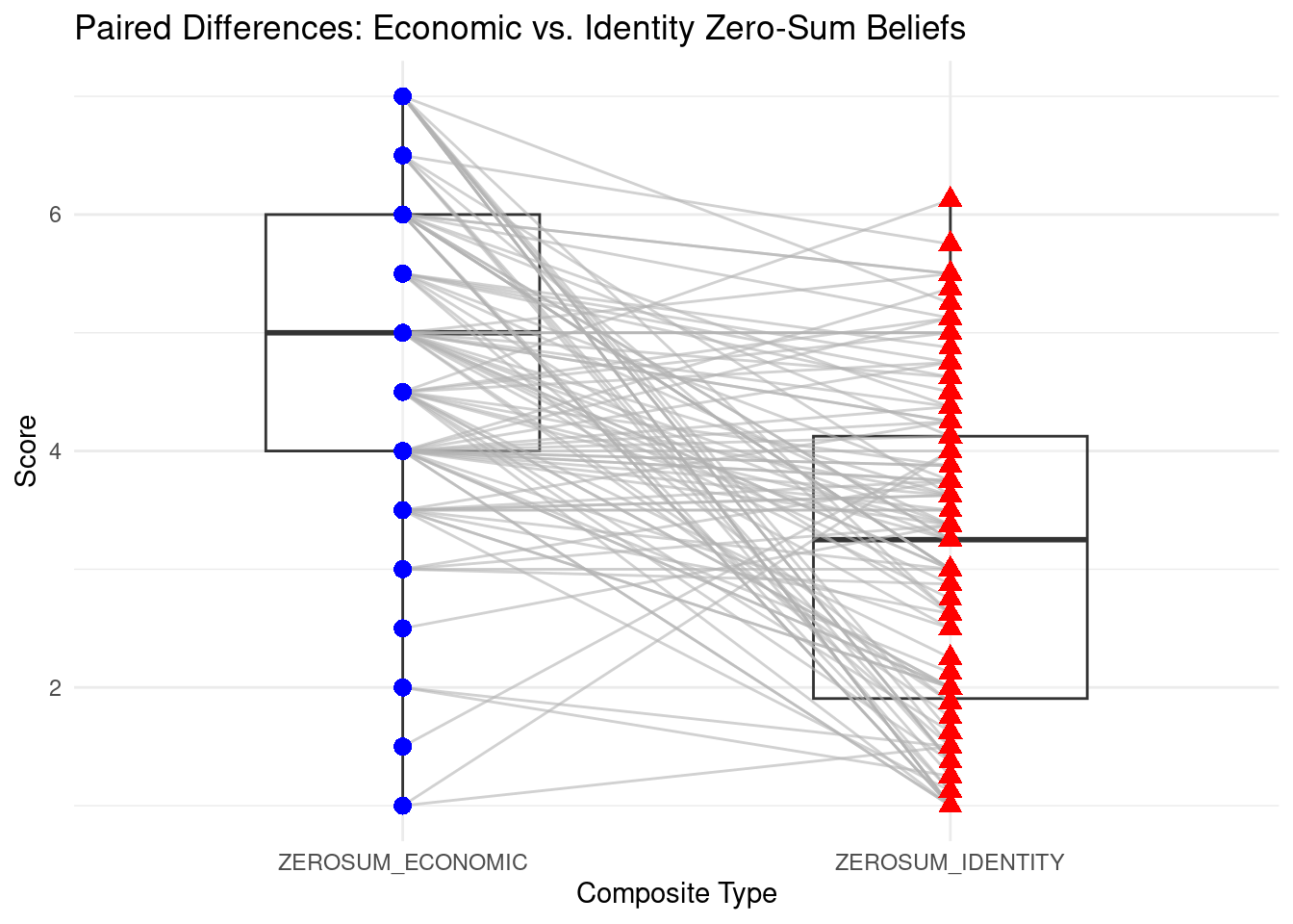
There is a significant difference between participants’ scores on ZEROSUM_ECONOMIC and ZEROSUM_IDENTITY. On average, participants rated economic zero-sum beliefs 1.75 points higher than identity zero-sum beliefs, 95% CI [1.38, 2.12].

In [17]:

# Create long data with participant ID
paired_data_long <- select_data %>%
  select(ZEROSUM_ECONOMIC, ZEROSUM_IDENTITY) %>%
  filter(!is.na(ZEROSUM_ECONOMIC) & !is.na(ZEROSUM_IDENTITY)) %>%  # Remove missing pairs
  mutate(ID = row_number()) %>%
  pivot_longer(cols = c(ZEROSUM_ECONOMIC, ZEROSUM_IDENTITY), 
               names_to = "Composite", 
               values_to = "Score")

# Plot: boxplot + paired lines
ggplot(paired_data_long, aes(x = Composite, y = Score, group = ID)) +
  geom_boxplot(aes(group = Composite), width = 0.5, alpha = 0.3, fill = "white", outlier.shape = NA) +
  geom_line(color = "gray70", alpha = 0.6) +  
  geom_point(data = paired_data_long %>% 
             filter(Composite == "ZEROSUM_ECONOMIC"), 
             shape = 16, size = 3, color = "blue") +
  geom_point(data = paired_data_long %>% 
             filter(Composite == "ZEROSUM_IDENTITY"),
             shape = 17, size = 3, color = "red") +   
  labs(title = "Paired Differences: Economic vs. Identity Zero-Sum Beliefs",
       x = "Composite Type", y = "Score") +
  theme_minimal()

The final sample reflected racial diversity, with participants identifying as White (n = 48), Black (n = 25), Mixed or Other (n = 25), and Asian (n = 24).

In [18]:

table(select_data$ETHNICITY)

      Asian       Black Mixed/Other       White 
         23          25          23          45 

## notice that the groups are unequal which is a problem for the ANOVA.
## TO DO: consider whether we should do a non-parametric approach

# SOURCE FOR DUMMY CODE
## https://stats.oarc.ucla.edu/other/mult-pkg/faq/general/faqwhat-is-dummy-coding/
## https://www.nathanwhudson.com/courses/methods/resources/10.%20Dummy%20Coding.pdf
## can you find an R specific example? 

In [19]:

#select_data[, c("RACE", "RACIALIDENTITY.4", "ETHNICITY")]

## Race (RACIALIDENTITY.4) was derived from the RACE item. Ethnicity was taken directly from the ETHNICITY item. As expected, these variables were not mutually exclusive, some respondents who identified their race as Mixed/Other reported ethnicity as White. 

## So race and ethnicity maybe are not forced to be logically consistent in many people’s minds, I think that's not an error, just like “mixed / biracial” people have multiple identities, and “White” in ethnicity sometimes is interpreted as “White Hispanic” or simply culturally white.

In [20]:

table(select_data$RACIALIDENTITY.4, select_data$ETHNICITY, useNA = "ifany")

             
              Asian Black Mixed/Other White
  Asian          22     0           0     0
  Black           0    25           3     0
  Mixed/Other     0     0          16     3
  White           1     0           4    42

In [21]:

party_colors <- c("Democrat" = "#0015BC", "Republican" = "#E9141D", "Independent" = "#732C7B")

Zero-Sum Beliefs by Gender

In [22]:

# Run t-tests using the dummy variable
zerosum_1_gender <- t.test(ZEROSUM_1 ~ GENDER_MALE, data = select_data)

kable(
  data.frame(
    t = zerosum_1_gender$statistic,
    df = zerosum_1_gender$parameter,
    p_value = zerosum_1_gender$p.value,
    mean_group_0 = zerosum_1_gender$estimate[1],
    mean_group_1 = zerosum_1_gender$estimate[2],
    mean_difference = zerosum_1_gender$estimate[1] - zerosum_1_gender$estimate[2],
    CI_lower = zerosum_1_gender$conf.int[1],
    CI_upper = zerosum_1_gender$conf.int[2]
  ),
  caption = "Table 22. Independent Samples t-Test: ZEROSUM_1 by Gender",
  digits = 3,
  booktabs = TRUE
)

Table 22. Independent Samples t-Test: ZEROSUM_1 by Gender

	t	df	p_value	mean_group_0	mean_group_1	mean_difference	CI_lower	CI_upper
t	0.964	111.94	0.337	4.086	3.776	0.31	-0.328	0.948

There is no significant difference in ZEROSUM_1 scores between men and women (p = .63). The difference in means is small and not statistically meaningful. The 95% CI (-0.48, 0.80) also includes zero, supporting the lack of difference.

In [23]:

ZEROSUM_ECONOMIC_gender <- t.test(ZEROSUM_ECONOMIC ~ GENDER_MALE, data = select_data)

kable(
  data.frame(
    t = ZEROSUM_ECONOMIC_gender$statistic,
    df = ZEROSUM_ECONOMIC_gender$parameter,
    p_value = ZEROSUM_ECONOMIC_gender$p.value,
    mean_group_0 = ZEROSUM_ECONOMIC_gender$estimate[1],
    mean_group_1 = ZEROSUM_ECONOMIC_gender$estimate[2],
    mean_difference = ZEROSUM_ECONOMIC_gender$estimate[1] - ZEROSUM_ECONOMIC_gender$estimate[2],
    CI_lower = ZEROSUM_ECONOMIC_gender$conf.int[1],
    CI_upper = ZEROSUM_ECONOMIC_gender$conf.int[2]
  ),
  caption = "Table 23. Independent Samples t-Test: ZEROSUM_ECONOMIC by Gender",
  digits = 3,
  booktabs = TRUE
)

Table 23. Independent Samples t-Test: ZEROSUM_ECONOMIC by Gender

	t	df	p_value	mean_group_0	mean_group_1	mean_difference	CI_lower	CI_upper
t	1.172	110.757	0.244	4.956	4.664	0.292	-0.202	0.787

There is no significant difference in ZEROSUM_ECONOMIC beliefs between men and women (p = .27). Although women’s mean score appears slightly higher, this difference is not statistically significant. The 95% CI (-0.21, 0.75) includes zero.

In [24]:

ZEROSUM_IDENTITY_gender <- t.test(ZEROSUM_IDENTITY ~ GENDER_MALE, data = select_data)

kable(
  data.frame(
    t = ZEROSUM_IDENTITY_gender$statistic,
    df = ZEROSUM_IDENTITY_gender$parameter,
    p_value = ZEROSUM_IDENTITY_gender$p.value,
    mean_group_0 = ZEROSUM_IDENTITY_gender$estimate[1],
    mean_group_1 = ZEROSUM_IDENTITY_gender$estimate[2],
    mean_difference = ZEROSUM_IDENTITY_gender$estimate[1] - ZEROSUM_IDENTITY_gender$estimate[2],
    CI_lower = ZEROSUM_IDENTITY_gender$conf.int[1],
    CI_upper = ZEROSUM_IDENTITY_gender$conf.int[2]
  ),
  caption = "Table 24. Independent Samples t-Test: ZEROSUM_IDENTITY by Gender",
  digits = 3,
  booktabs = TRUE
)

Table 24. Independent Samples t-Test: ZEROSUM_IDENTITY by Gender

	t	df	p_value	mean_group_0	mean_group_1	mean_difference	CI_lower	CI_upper
t	-0.093	111.232	0.926	3.105	3.129	-0.024	-0.541	0.492

There is no significant difference in ZEROSUM_IDENTITY beliefs between men and women (p = .92). The near-zero difference and very wide p-value indicate no group difference at all.

In [25]:

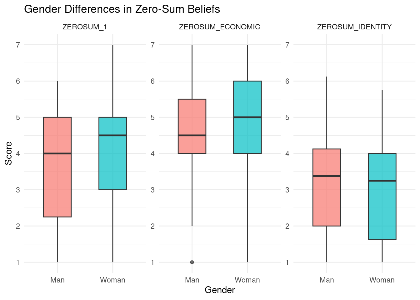
# Reshape the data to long format for easier plotting
long_data <- select_data %>%
  select(GENDER_MALE, ZEROSUM_1, ZEROSUM_ECONOMIC, ZEROSUM_IDENTITY) %>%
  mutate(GENDER = ifelse(GENDER_MALE == 1, "Man", "Woman")) %>%
  pivot_longer(cols = c(ZEROSUM_1, ZEROSUM_ECONOMIC, ZEROSUM_IDENTITY),
               names_to = "Variable",
               values_to = "Score")

# Create boxplots
ggplot(long_data, aes(x = GENDER, y = Score, fill = GENDER)) +
  geom_boxplot(width = 0.5, alpha = 0.7) +
  facet_wrap(~ Variable, scales = "free_y") +
  labs(title = "Gender Differences in Zero-Sum Beliefs",
       x = "Gender",
       y = "Score") +
  scale_y_continuous(limits = c(1, 7), breaks = 1:7) +
  theme_minimal() +
  theme(legend.position = "none")

Warning: Removed 3 rows containing non-finite outside the scale range
(`stat_boxplot()`).

Across all three variables (ZEROSUM_1, ZEROSUM_ECONOMIC, ZEROSUM_IDENTITY), gender is not associated with significant differences in zero-sum beliefs in our sample. As shown in the box plots, the median scores are nearly identical across genders, and the range from the median to the 3rd quartile (i.e., the upper half of the middle 50%) is also highly similar. The overall range of scores tends to span from approximately 1 to 7 for both female and male participants, further indicating that the distribution of zero-sum beliefs is comparable across gender groups.

Zero-Sum Beliefs by Political Party Affiliation

Gain vs. Loss

Do zero-sum beliefs regarding gains and losses differ by racial/ethnic identity and political party affiliation?

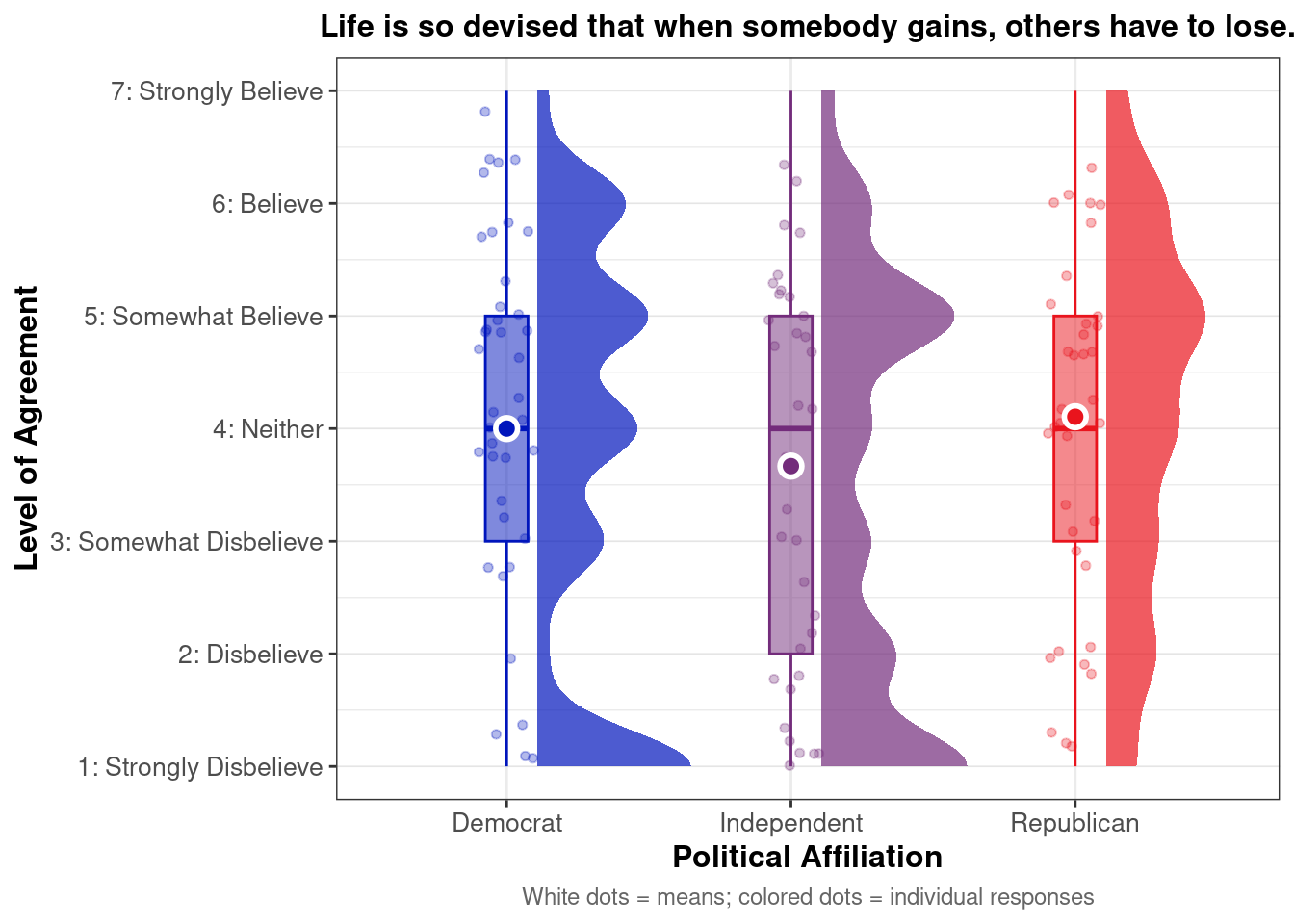
Below we present descriptive statistics and visualizations for ZEROSUM_1 (“Life is so devised that when somebody gains, others have to lose”), examining how responses vary across racial identity and political affiliation.

In [26]:

library(dplyr)
group_stats_1 <- select_data %>%
  group_by(POLITICALPARTY, RACIALIDENTITY.4) %>%
  summarise(
    mean_ZEROSUM_1 = mean(ZEROSUM_1, na.rm = TRUE),
    se = sd(ZEROSUM_1, na.rm = TRUE) / sqrt(n()),
    .groups = 'drop'
  )

# Check the structure
#str(group_stats_1)

In [27]:

head(group_stats_1)

# A tibble: 6 × 4
  POLITICALPARTY RACIALIDENTITY.4 mean_ZEROSUM_1    se
  <chr>          <chr>                     <dbl> <dbl>
1 Democrat       Asian                      4.25 0.491
2 Democrat       Black                      4.5  0.5  
3 Democrat       Mixed/Other                3.29 0.474
4 Democrat       White                      3.88 0.514
5 Independent    Asian                      3    0.617
6 Independent    Black                      3.75 0.75 

In [28]:

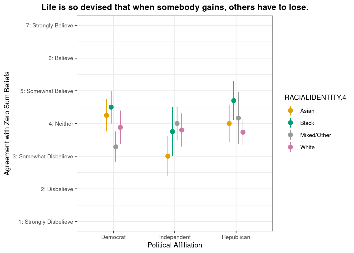
# Define the zesty_four palette
zesty_four <- c("#E69F00", "#009E73", "#999999", "#CC79A7") 

# Create the plot with pointrange
plot.zerosum1 <- ggplot(group_stats_1, aes(POLITICALPARTY, mean_ZEROSUM_1)) +
  geom_pointrange(aes(color = RACIALIDENTITY.4, 
                      ymin = mean_ZEROSUM_1 - se,  # Use standard error instead of sd
                      ymax = mean_ZEROSUM_1 + se), # Use standard error instead of sd
                  position = position_dodge(0.3)) +
  theme_bw() +
  labs(title = "Life is so devised that when somebody gains, others have to lose.",
       x = "Political Affiliation",
       y = "Agreement with Zero Sum Beliefs",
       color = "RACIALIDENTITY.4") + 
  theme(
    plot.title = element_text(size = 12, face = "bold", hjust = 0.5),
    axis.title = element_text(size = 10),
    axis.text = element_text(size = 8),
    legend.title = element_text(size = 10),
    legend.text = element_text(size = 8)
  ) +
  scale_y_continuous(
    breaks = 1:7,
    labels = c("1: Strongly Disbelieve", 
               "2: Disbelieve", 
               "3: Somewhat Disbelieve", 
               "4: Neither", 
               "5: Somewhat Believe", 
               "6: Believe", 
               "7: Strongly Believe"),
    limits = c(1, 7)  # Set the y-axis limits to match the scale
  )+
  scale_color_manual(values = zesty_four)

# Print and save the plots
print(plot.zerosum1)

Mean agreement with the belief that “life is so devised that when somebody gains, others have to lose,” by political party and racial/ethnic identity.

ggsave("plots/plot1:gain-lose.png", 
       plot = plot.zerosum1, 
       width = 10, 
       height = 8, 
       dpi = 300)

This pointrange plot shows that Black respondents exhibit higher agreement with the belief that “life is so devised that when somebody gains, others have to lose” among Republicans and Democrats, highlighting group-based differences in zero-sum beliefs.

In [29]:

# ZEROSUM_1 average score with 95% CI
group_stats_1_avg <- select_data %>%
  group_by(POLITICALPARTY) %>%
  summarise(
    mean_ZEROSUM_1 = mean(ZEROSUM_1, na.rm = TRUE),
    se = sd(ZEROSUM_1, na.rm = TRUE) / sqrt(n()),
    n = n(),
    .groups = 'drop'
  ) %>%
  mutate(
    # Calculate 95% confidence interval using t-distribution
    t_value = qt(0.975, df = n - 1),  # 95% CI, two-tailed
    ci_lower = mean_ZEROSUM_1 - t_value * se,
    ci_upper = mean_ZEROSUM_1 + t_value * se
  )

Do zero-sum beliefs regarding gains and losses differ by political party affiliation?

In [30]:

library(ggdist)
library(patchwork)

plot.zerosum1_raincloud <- select_data %>%
  filter(!is.na(ZEROSUM_1), !is.na(POLITICALPARTY)) %>%
  ggplot(aes(x = POLITICALPARTY, y = ZEROSUM_1, fill = POLITICALPARTY, color = POLITICALPARTY)) +
  stat_halfeye(
    adjust = 0.5,
    width = 0.6,
    .width = 0,
    justification = -0.2,
    point_colour = NA,
    alpha = 0.7
  ) +
  geom_boxplot(
    width = 0.15,
    outlier.shape = NA,
    alpha = 0.5
  ) +
  geom_point(
    size = 1.3,
    alpha = 0.3,
    position = position_jitter(
      seed = 1, width = 0.1
    )
  ) +
  stat_summary(
    fun = mean,
    geom = "point",
    size = 3,
    color = "white",
    stroke = 1.5,
    shape = 21
  ) +
  scale_fill_manual(values = party_colors) +
  scale_color_manual(values = party_colors) +
  theme_bw() +
  labs(
    title = "Life is so devised that when somebody gains, others have to lose.",
    x = "Political Affiliation",
    y = "Level of Agreement",
    caption = "White dots = means; colored dots = individual responses"
  ) +
  theme(
    plot.title = element_text(size = 12, face = "bold", hjust = 0.5),
    plot.caption = element_text(size = 9, color = "gray40", hjust = 0.5),
    axis.title = element_text(size = 12, face = "bold"),
    axis.text = element_text(size = 10),
    legend.position = "none",
    panel.grid.major.y = element_line(color = "gray90", linewidth = 0.3)  # Fixed
  ) +
  scale_y_continuous(
    breaks = 1:7,
    labels = c("1: Strongly Disbelieve", 
               "2: Disbelieve", 
               "3: Somewhat Disbelieve", 
               "4: Neither", 
               "5: Somewhat Believe", 
               "6: Believe", 
               "7: Strongly Believe"),
    limits = c(1, 7) 
  )

plot.zerosum1_raincloud

Warning: Removed 6 rows containing missing values or values outside the scale range
(`geom_point()`).

Distribution of agreement with ‘life is so devised that when somebody gains, others have to lose’ by political affiliation. White dots represent means; colored dots are individual responses.

This raincloud plot shows that mean agreement with the zero-sum belief (indicated by white dots) varies by political affiliation. Among the three groups, Republicans exhibit higher average agreement with the statement “Life is so devised that when somebody gains, others have to lose.” The distribution (via density and individual dots) suggests greater clustering of high agreement scores among partisans, reflecting perceived competition between social groups. The relatively narrow IQRs and tight clustering around high values also indicate consistent endorsement of this belief within parties.

In [31]:

shapiro_zerosum1 <- select_data %>%
  group_by(RACIALIDENTITY.4) %>%
  summarise(p = shapiro.test(ZEROSUM_1)$p.value)

kable(
  shapiro_zerosum1,
  caption = "Table 25. Shapiro–Wilk Normality Test for ZEROSUM_1 by Racial Identity",
  digits = 4,
  booktabs = TRUE
)

Table 25. Shapiro–Wilk Normality Test for ZEROSUM_1 by Racial Identity

RACIALIDENTITY.4	p
Asian	0.0758
Black	0.0143
Mixed/Other	0.1651
White	0.0002

## White, Mixed/Other (p<0.05) fail the normality assumption for ANOVA, maybe use a non-parametric test (Kruskal-Wallis)

In [32]:

library(tibble)
library(rempsyc)
library(kableExtra)

kw.ZEROSUM_1.party <- kruskal.test(ZEROSUM_1 ~ POLITICALPARTY, data = select_data)

kw_table <- tibble(
  Predictor = c("POLITICALPARTY"),
  df = c(length(unique(select_data$POLITICALPARTY)) - 1),
  `Chi-squared` = c(round(kw.ZEROSUM_1.party$statistic, 2)),
  p = c(round(kw.ZEROSUM_1.party$p.value, 3))
)

if (knitr::is_html_output()) {
  kw_table %>%
    knitr::kable(
      digits = 3,
      escape = TRUE,
      format = "html",
      caption = "Table 26. Kruskal-Wallis Test Results for ZEROSUM_1"
    ) %>%
    kableExtra::kable_styling(bootstrap_options = c("striped", "hover", "condensed")) %>%
    kableExtra::row_spec(
      which(kw_table$p < 0.05), 
      background = "gray"
    )
} else if (knitr::is_latex_output()) {
  kw_table %>%
    knitr::kable(
      digits = 3,
      escape = TRUE,
      format = "latex",
      longtable = TRUE,
      caption = "Kruskal-Wallis Test Results for ZEROSUM\\_1"
    ) %>%
    kableExtra::kable_styling(full_width = FALSE, position = "left") %>%
    kableExtra::row_spec(
      which(kw_table$p < 0.05), 
      background = "gray!20"
    )
}

Table 26. Kruskal-Wallis Test Results for ZEROSUM_1

Predictor	df	Chi-squared	p
POLITICALPARTY	2	1.04	0.594

There was no significant difference in ZEROSUM_1 scores across political party groups, Kruskal-Wallis χ²(2) = 1.04, p = 0.594.

Poor vs. Rich

Do zero-sum beliefs regarding poor and rich differ by racial/ethnic identity and political party affiliation?

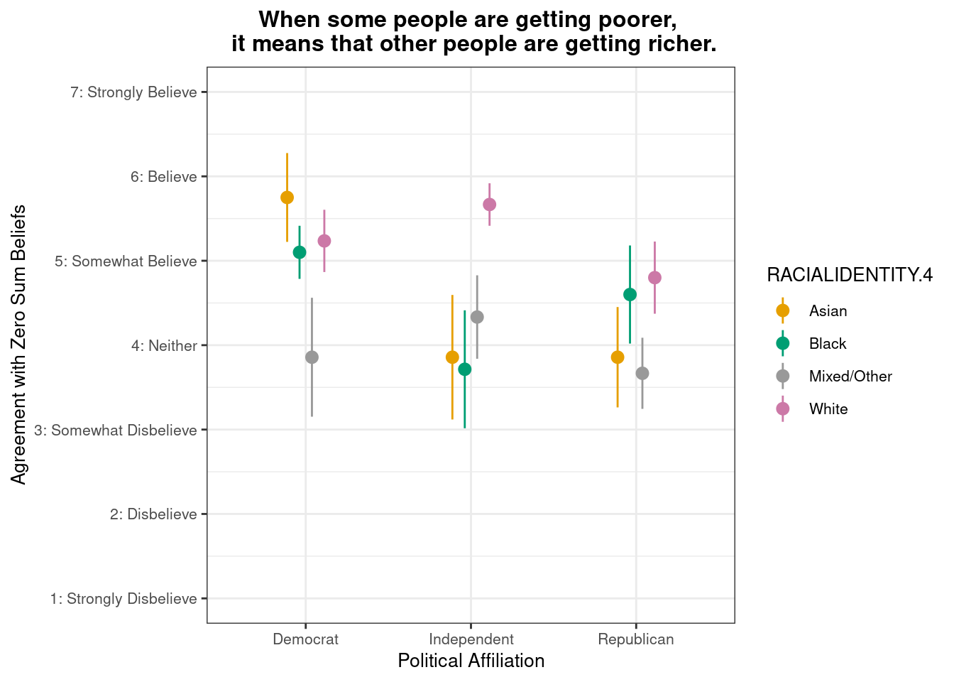
Below we present descriptive statistics and visualizations for ZEROSUM_2 (“When some people are getting poorer, it means that other people are getting richer.”), examining how responses vary across racial identity and political affiliation.

In [33]:

library(dplyr)
group_stats_2 <- select_data %>%
  group_by(POLITICALPARTY, RACIALIDENTITY.4) %>%
  summarise(
    mean_ZEROSUM_2 = mean(ZEROSUM_2, na.rm = TRUE),
    se = sd(ZEROSUM_2, na.rm = TRUE) / sqrt(n()),
    .groups = 'drop'
  )

# Check the structure
#str(group_stats_2)

In [34]:

head(group_stats_2)

# A tibble: 6 × 4
  POLITICALPARTY RACIALIDENTITY.4 mean_ZEROSUM_2    se
  <chr>          <chr>                     <dbl> <dbl>
1 Democrat       Asian                      5.75 0.526
2 Democrat       Black                      5.1  0.314
3 Democrat       Mixed/Other                3.86 0.705
4 Democrat       White                      5.24 0.369
5 Independent    Asian                      3.86 0.738
6 Independent    Black                      3.71 0.699

In [35]:

# Define the zesty_four palette
zesty_four <- c("#E69F00", "#009E73", "#999999", "#CC79A7") 

# Create the plot with pointrange
plot.zerosum2 <- ggplot(group_stats_2, 
                        aes(POLITICALPARTY, mean_ZEROSUM_2)) +
  geom_pointrange(aes(color = RACIALIDENTITY.4,
                      ymin = mean_ZEROSUM_2 - se,
                      # Use standard error instead of sd
                      ymax = mean_ZEROSUM_2 + se),
                      # Use standard error instead of sd
                      position = position_dodge(0.3)) +
  theme_bw() +
  labs(title = "When some people are getting poorer, \n it means that other people are getting richer.",
       x = "Political Affiliation",
       y = "Agreement with Zero Sum Beliefs",
       color = "RACIALIDENTITY.4") + 
  theme(
    plot.title = element_text(size = 12, face = "bold", hjust = 0.5),
    axis.title = element_text(size = 10),
    axis.text = element_text(size = 8),
    legend.title = element_text(size = 10),
    legend.text = element_text(size = 8)
  ) +
  scale_y_continuous(
    breaks = 1:7,
    labels = c("1: Strongly Disbelieve", 
               "2: Disbelieve", 
               "3: Somewhat Disbelieve", 
               "4: Neither", 
               "5: Somewhat Believe", 
               "6: Believe", 
               "7: Strongly Believe"),
    limits = c(1, 7)  # Set the y-axis limits to match the scale
  )+
  scale_color_manual(values = zesty_four)

# Print and save the plots
print(plot.zerosum2)

ggsave("plots/plot2:poor-rich.png", 
       plot = plot.zerosum2, 
       width = 10, 
       height = 8, 
       dpi = 300)

This pointrange plot shows that White respondents exhibit higher agreement with the belief that “when some people are getting poorer, it means that other people are getting richer” among Republicans and Independents, highlighting group-based differences in zero-sum beliefs.

In [36]:

# ZEROSUM_1 average score with 95% CI
group_stats_2_avg <- select_data %>%
  group_by(POLITICALPARTY) %>%
  summarise(
    mean_ZEROSUM_2 = mean(ZEROSUM_2, na.rm = TRUE),
    se = sd(ZEROSUM_2, na.rm = TRUE) / sqrt(n()),
    n = n(),
    .groups = 'drop'
  ) %>%
  mutate(
    # Calculate 95% confidence interval using t-distribution
    t_value = qt(0.975, df = n - 1),  # 95% CI, two-tailed
    ci_lower = mean_ZEROSUM_2 - t_value * se,
    ci_upper = mean_ZEROSUM_2 + t_value * se
  )

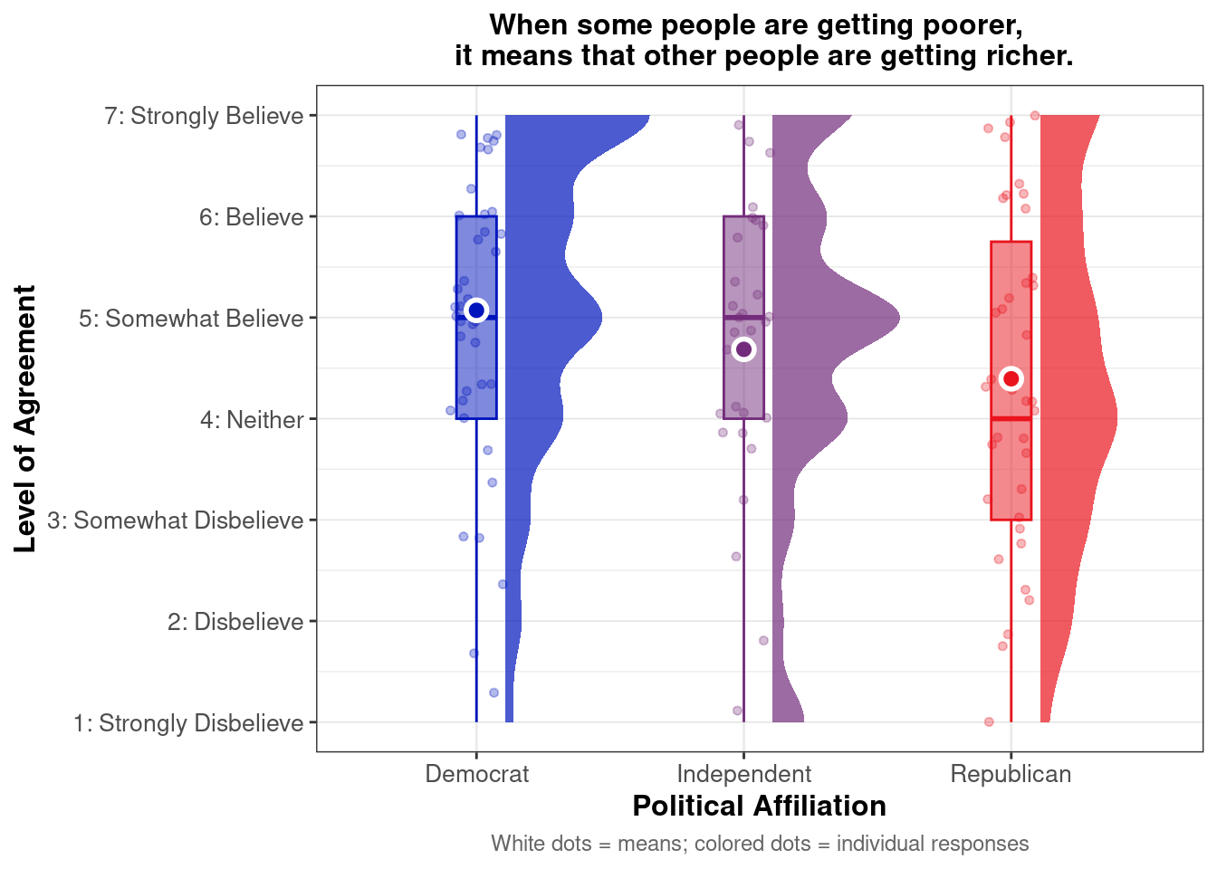
Do zero-sum beliefs regarding poor and rich differ by political party affiliation?

In [37]:

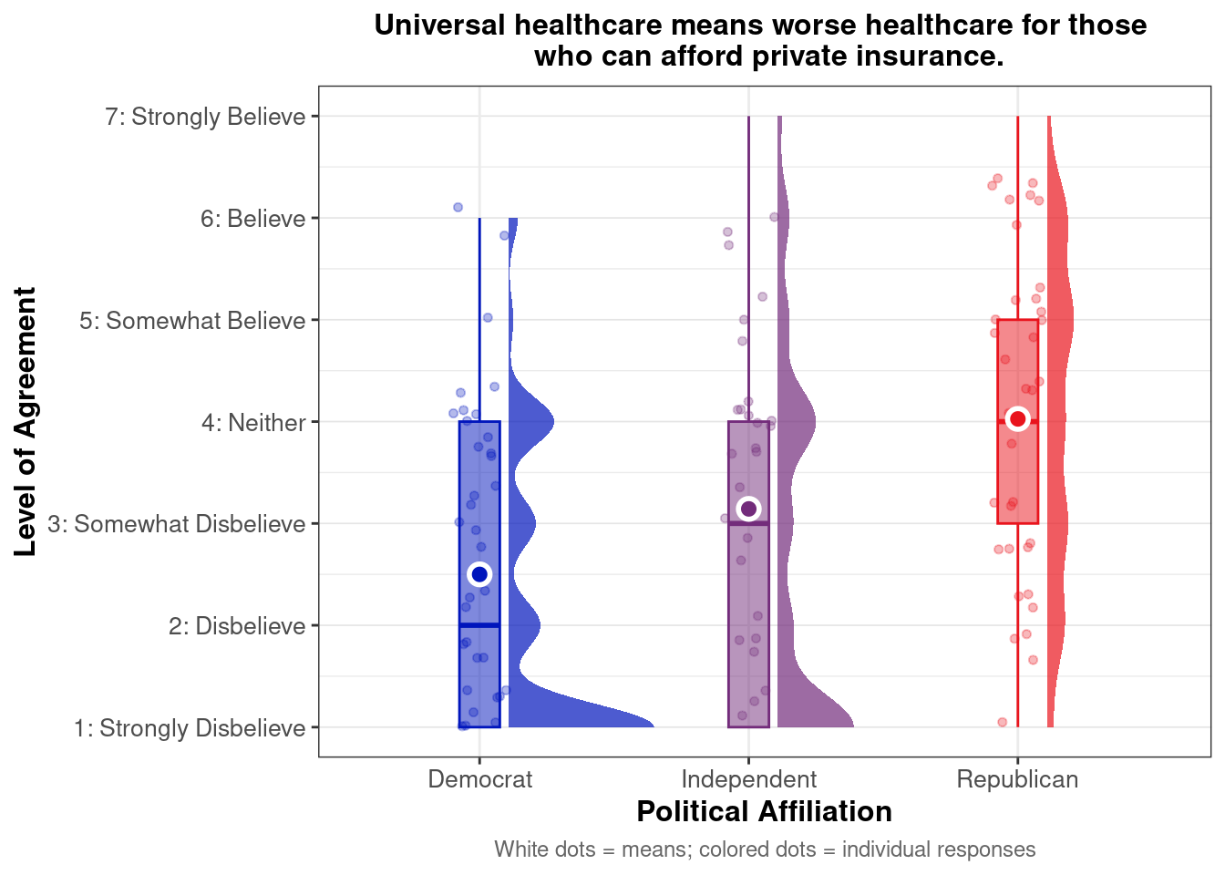
library(ggdist)
library(patchwork)

plot.zerosum2_raincloud <- select_data %>%
  filter(!is.na(ZEROSUM_2), !is.na(POLITICALPARTY)) %>%
  ggplot(aes(x = POLITICALPARTY, y = ZEROSUM_2, fill = POLITICALPARTY, color = POLITICALPARTY)) +
  stat_halfeye(
    adjust = 0.5,
    width = 0.6,
    .width = 0,
    justification = -0.2,
    point_colour = NA,
    alpha = 0.7
  ) +
  geom_boxplot(
    width = 0.15,
    outlier.shape = NA,
    alpha = 0.5
  ) +
  geom_point(
    size = 1.3,
    alpha = 0.3,
    position = position_jitter(
      seed = 1, width = 0.1
    )
  ) +
  stat_summary(
    fun = mean,
    geom = "point",
    size = 3,
    color = "white",
    stroke = 1.5,
    shape = 21
  ) +
  scale_fill_manual(values = party_colors) +
  scale_color_manual(values = party_colors) +
  theme_bw() +
  labs(
    title = "When some people are getting poorer, \n it means that other people are getting richer.",
    x = "Political Affiliation",
    y = "Level of Agreement",
    caption = "White dots = means; colored dots = individual responses"
  ) +
  theme(
    plot.title = element_text(size = 12, face = "bold", hjust = 0.5),
    plot.caption = element_text(size = 9, color = "gray40", hjust = 0.5),
    axis.title = element_text(size = 12, face = "bold"),
    axis.text = element_text(size = 10),
    legend.position = "none",
    panel.grid.major.y = element_line(color = "gray90", linewidth = 0.3)  # Fixed
  ) +
  scale_y_continuous(
    breaks = 1:7,
    labels = c("1: Strongly Disbelieve", 
               "2: Disbelieve", 
               "3: Somewhat Disbelieve", 
               "4: Neither", 
               "5: Somewhat Believe", 
               "6: Believe", 
               "7: Strongly Believe"),
    limits = c(1, 7) 
  )
plot.zerosum2_raincloud

Warning: Removed 8 rows containing missing values or values outside the scale range
(`geom_point()`).

This raincloud plot shows that mean agreement with the zero-sum belief (indicated by white dots) varies by political affiliation. Among the three groups, Democrat exhibit higher average agreement with the statement “When some people are getting poorer, it means that other people are getting richer.” ßThe distribution (via density and individual dots) reveals different patterns across groups. Democrats show greater clustering of high agreement scores (concentrated in the 5-7 range). Republicans show the most dispersed distribution with responses spread across nearly the full scale. Independents are more concentrated in the middle-to-lower range.

In [38]:

shapiro_zerosum2 <- select_data %>%
  group_by(RACIALIDENTITY.4) %>%
  summarise(p = shapiro.test(ZEROSUM_2)$p.value)

kable(
  shapiro_zerosum2,
  caption = "Table 27. Shapiro–Wilk Normality Test for ZEROSUM_2 by Racial Identity",
  digits = 4,
  booktabs = TRUE
)

Table 27. Shapiro–Wilk Normality Test for ZEROSUM_2 by Racial Identity

RACIALIDENTITY.4	p
Asian	0.0203
Black	0.0410
Mixed/Other	0.1886
White	0.0005

## Asian, Black, White (p<0.05) fail the normality assumption for ANOVA, maybe use a non-parametric test (Kruskal-Wallis)

In [39]:

library(tibble)
library(knitr)
library(kableExtra)

kw.ZEROSUM_2.party <- kruskal.test(ZEROSUM_2 ~ POLITICALPARTY, data = select_data)

kw_table <- tibble(
  Predictor = c("POLITICALPARTY"),
  df = c(length(unique(select_data$POLITICALPARTY)) - 1),
  `Chi-squared` = c(round(kw.ZEROSUM_2.party$statistic, 2)),
  p = c(round(kw.ZEROSUM_2.party$p.value, 3))
)

if (knitr::is_html_output()) {
  kw_table %>%
    knitr::kable(
      digits = 3,
      escape = TRUE,
      format = "html",
      caption = "Table 28. Kruskal-Wallis Test Results for ZEROSUM_2"
    ) %>%
    kableExtra::kable_styling(bootstrap_options = c("striped", "hover", "condensed")) %>%
    kableExtra::row_spec(
      which(kw_table$p < 0.05),
      background = "gray"
    )
} else if (knitr::is_latex_output()) {
  kw_table %>%
    knitr::kable(
      digits = 3,
      escape = TRUE,
      format = "latex",
      longtable = TRUE,
      caption = "Kruskal-Wallis Test Results for ZEROSUM\\_2"
    ) %>%
    kableExtra::kable_styling(full_width = FALSE, position = "left") %>%
    kableExtra::row_spec(
      which(kw_table$p < 0.05),
      background = "gray!20"
    )
}

Table 28. Kruskal-Wallis Test Results for ZEROSUM_2

Predictor	df	Chi-squared	p
POLITICALPARTY	2	4.09	0.129

There was no significant difference in ZEROSUM_2 scores across political party groups, Kruskal-Wallis χ²(2) = 4.09, p = 0.129.

Wealth few vs. many

Do zero-sum beliefs regarding wealth concentration differ by racial/ethnic identity and political party affiliation?

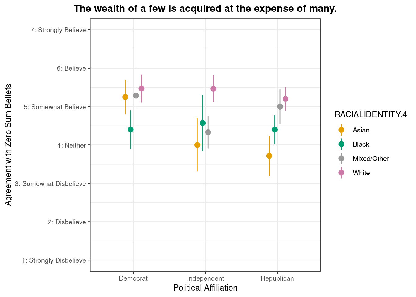
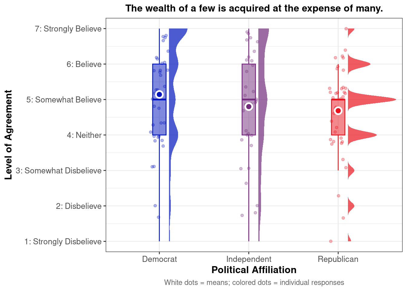
Below we present descriptive statistics and visualizations for ZEROSUM_3 (“The wealth of a few is acquired at the expense of many.”), examining how responses vary across racial identity and political affiliation.

In [40]:

library(dplyr)
group_stats_3 <- select_data %>%
  group_by(POLITICALPARTY, RACIALIDENTITY.4) %>%
  summarise(
    mean_ZEROSUM_3 = mean(ZEROSUM_3, na.rm = TRUE),
    se = sd(ZEROSUM_3, na.rm = TRUE) / sqrt(n()),
    .groups = 'drop'
  )

# Check the structure
#str(group_stats_3)

In [41]:

head(group_stats_3)

# A tibble: 6 × 4
  POLITICALPARTY RACIALIDENTITY.4 mean_ZEROSUM_3    se
  <chr>          <chr>                     <dbl> <dbl>
1 Democrat       Asian                      5.25 0.453
2 Democrat       Black                      4.4  0.499
3 Democrat       Mixed/Other                5.29 0.747
4 Democrat       White                      5.47 0.365
5 Independent    Asian                      4    0.690
6 Independent    Black                      4.57 0.732

In [42]:

# Define the zesty_four palette
zesty_four <- c("#E69F00", "#009E73", "#999999", "#CC79A7") 

# Create the plot with pointrange
plot.zerosum3 <- ggplot(group_stats_3,
                        aes(POLITICALPARTY, mean_ZEROSUM_3)) +
  geom_pointrange(aes(color = RACIALIDENTITY.4,
                      ymin = mean_ZEROSUM_3 - se,
                      # Use standard error instead of sd
                      ymax = mean_ZEROSUM_3 + se),
                      # Use standard error instead of sd
                      position = position_dodge(0.3)) +
  theme_bw() +
  labs(title = "The wealth of a few is acquired at the expense of many.",
       x = "Political Affiliation",
       y = "Agreement with Zero Sum Beliefs",
       color = "RACIALIDENTITY.4") + 
  theme(
    plot.title = element_text(size = 12, face = "bold", hjust = 0.5),
    axis.title = element_text(size = 10),
    axis.text = element_text(size = 8),
    legend.title = element_text(size = 10),
    legend.text = element_text(size = 8)
  ) +
  scale_y_continuous(
    breaks = 1:7,
    labels = c("1: Strongly Disbelieve", 
               "2: Disbelieve", 
               "3: Somewhat Disbelieve", 
               "4: Neither", 
               "5: Somewhat Believe", 
               "6: Believe", 
               "7: Strongly Believe"),
    limits = c(1, 7)  # Set the y-axis limits to match the scale
  )+
  scale_color_manual(values = zesty_four)

# Print and save the plots
print(plot.zerosum3)

ggsave("plots/plot3:wealthfew-many.png", 
       plot = plot.zerosum3, 
       width = 10, 
       height = 8, 
       dpi = 300)

This pointrange plot shows that White respondents exhibit higher agreement with the belief that “the wealth of a few is acquired at the expense of many” among all three political groups, highlighting group-based differences in zero-sum beliefs.

In [43]:

# ZEROSUM_3 average score with 95% CI
group_stats_3_avg <- select_data %>%
  group_by(POLITICALPARTY) %>%
  summarise(
    mean_ZEROSUM_3 = mean(ZEROSUM_3, na.rm = TRUE),
    se = sd(ZEROSUM_3, na.rm = TRUE) / sqrt(n()),
    n = n(),
    .groups = 'drop'
  ) %>%
  mutate(
    # Calculate 95% confidence interval using t-distribution
    t_value = qt(0.975, df = n - 1),  # 95% CI, two-tailed
    ci_lower = mean_ZEROSUM_3 - t_value * se,
    ci_upper = mean_ZEROSUM_3 + t_value * se
  )

Do zero-sum beliefs regarding wealth concentration differ by political party affiliation?

In [44]:

plot.zerosum3_raincloud <- select_data %>%
  filter(!is.na(ZEROSUM_3), !is.na(POLITICALPARTY)) %>%
  ggplot(aes(x = POLITICALPARTY, y = ZEROSUM_3, fill = POLITICALPARTY, color = POLITICALPARTY)) +
  stat_halfeye(
    adjust = 0.5,
    width = 0.6,
    .width = 0,
    justification = -0.2,
    point_colour = NA,
    alpha = 0.7
  ) +
   geom_boxplot(
    width = 0.15,
    outlier.shape = NA,
    alpha = 0.5
  ) +
  geom_point(
    size = 1.3,
    alpha = 0.3,
    position = position_jitter(
      seed = 1, width = 0.1
    )
  ) +
  stat_summary(
    fun = mean,
    geom = "point",
    size = 3,
    color = "white",
    stroke = 1.5,
    shape = 21
  ) +
  scale_fill_manual(values = party_colors) +
  scale_color_manual(values = party_colors) +
  theme_bw() +
  labs(
    title = "The wealth of a few is acquired at the expense of many.",
    x = "Political Affiliation",
    y = "Level of Agreement",
    caption = "White dots = means; colored dots = individual responses"
  ) +
  theme(
    plot.title = element_text(size = 12, face = "bold", hjust = 0.5),
    plot.caption = element_text(size = 9, color = "gray40", hjust = 0.5),
    axis.title = element_text(size = 12, face = "bold"),
    axis.text = element_text(size = 10),
    legend.position = "none",
    panel.grid.major.y = element_line(color = "gray90", linewidth = 0.3)  # Fixed
  ) +
  scale_y_continuous(
    breaks = 1:7,
    labels = c("1: Strongly Disbelieve", 
               "2: Disbelieve", 
               "3: Somewhat Disbelieve", 
               "4: Neither", 
               "5: Somewhat Believe", 
               "6: Believe", 
               "7: Strongly Believe"),
    limits = c(1, 7) 
  )
plot.zerosum3_raincloud

Warning: Removed 10 rows containing missing values or values outside the scale range
(`geom_point()`).

This raincloud plot shows that mean agreement with the zero-sum belief (indicated by white dots) varies by political affiliation. Among the three groups, Democrat exhibit higher average agreement with the statement “the wealth of a few is acquired at the expense of many.” The distribution (via density and individual dots) reveals different patterns across groups. Democrats show strong clustering around high agreement scores (concentrated in the 5-7 range) with a clear rightward skew toward stronger belief. Republicans display a more spread distribution with notable presence across moderate to high agreement levels, though still centered around the middle range. Independents show a relatively concentrated distribution around the moderate-to-high range (4-6), with their mean falling between the other two groups.

In [45]:

shapiro_zerosum3 <- select_data %>%
  group_by(RACIALIDENTITY.4) %>%
  summarise(p = shapiro.test(ZEROSUM_3)$p.value)

kable(
  shapiro_zerosum3,
  caption = "Table 29. Shapiro–Wilk Normality Test for ZEROSUM_3 by Racial Identity",
  digits = 6,
  booktabs = TRUE
)

Table 29. Shapiro–Wilk Normality Test for ZEROSUM_3 by Racial Identity

RACIALIDENTITY.4	p
Asian	0.176619
Black	0.031488
Mixed/Other	0.031972
White	0.000089

## Black, White, Mixed/Other (p<0.05) fail the normality assumption for ANOVA, maybe use a non-parametric test (Kruskal-Wallis)

In [46]:

library(tibble)
library(rempsyc)

kw.ZEROSUM_3.party <- kruskal.test(ZEROSUM_3 ~ POLITICALPARTY, data = select_data)

kw_table <- tibble(
  Predictor = c("POLITICALPARTY"),
  df = c(length(unique(select_data$POLITICALPARTY)) - 1),
  `Chi-squared` = c(round(kw.ZEROSUM_3.party$statistic, 2)),
  p = c(round(kw.ZEROSUM_3.party$p.value, 3))
)

if (knitr::is_html_output()) {
  kw_table %>%
    knitr::kable(
      digits = 3,
      escape = TRUE,
      format = "html",
      caption = "Table 30. Kruskal-Wallis Test Results for ZEROSUM_3"
    ) %>%
    kableExtra::kable_styling(bootstrap_options = c("striped", "hover", "condensed")) %>%
    kableExtra::row_spec(
      which(kw_table$p < 0.05),
      background = "gray"
    )
} else if (knitr::is_latex_output()) {
  kw_table %>%
    knitr::kable(
      digits = 3,
      escape = TRUE,
      format = "latex",
      longtable = TRUE,
      caption = "Kruskal-Wallis Test Results for ZEROSUM\\_3"
    ) %>%
    kableExtra::kable_styling(full_width = FALSE, position = "left") %>%
    kableExtra::row_spec(
      which(kw_table$p < 0.05),
      background = "gray!20"
    )
}

Table 30. Kruskal-Wallis Test Results for ZEROSUM_3

Predictor	df	Chi-squared	p
POLITICALPARTY	2	2.34	0.311

There was no significant difference in ZEROSUM_3 scores across political party groups, Kruskal-Wallis χ²(2) = 2.34, p = 0.311.

Women vs. Men

Do zero-sum beliefs regarding gender discrimination differ by racial/ethnic identity and political party affiliation?

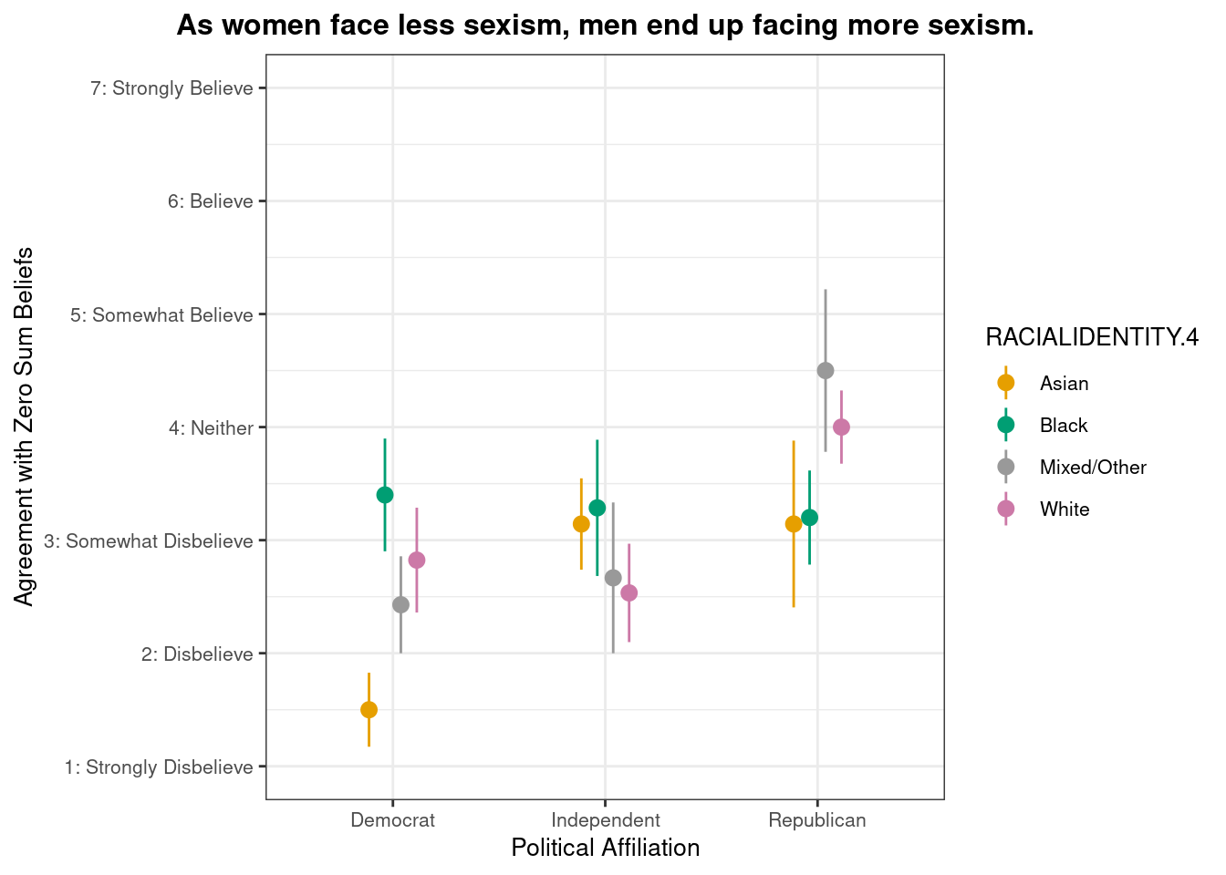
Below we present descriptive statistics and visualizations for ZEROSUM_4 (“As women face less sexism, men end up facing more sexism.”), examining how responses vary across racial identity and political affiliation.

In [47]:

library(dplyr)
group_stats_4 <- select_data %>%
  group_by(POLITICALPARTY, RACIALIDENTITY.4) %>%
  summarise(
    mean_ZEROSUM_4 = mean(ZEROSUM_4, na.rm = TRUE),
    se = sd(ZEROSUM_4, na.rm = TRUE) / sqrt(n()),
    .groups = 'drop'
  )

# Check the structure
#str(group_stats_4)

In [48]:

head(group_stats_4)

# A tibble: 6 × 4
  POLITICALPARTY RACIALIDENTITY.4 mean_ZEROSUM_4    se
  <chr>          <chr>                     <dbl> <dbl>
1 Democrat       Asian                      1.5  0.327
2 Democrat       Black                      3.4  0.499
3 Democrat       Mixed/Other                2.43 0.429
4 Democrat       White                      2.82 0.464
5 Independent    Asian                      3.14 0.404
6 Independent    Black                      3.29 0.603

In [49]:

# Define the zesty_four palette
zesty_four <- c("#E69F00", "#009E73", "#999999", "#CC79A7") 

# Create the plot with pointrange
plot.zerosum4 <- ggplot(group_stats_4, aes(POLITICALPARTY,
                                           mean_ZEROSUM_4)) +
  geom_pointrange(aes(color = RACIALIDENTITY.4, 
                      ymin = mean_ZEROSUM_4 - se,
                      # Use standard error instead of sd
                      ymax = mean_ZEROSUM_4 + se),
                      # Use standard error instead of sd
                      position = position_dodge(0.3)) +
  theme_bw() +
  labs(title = "As women face less sexism, men end up facing more sexism.",
       x = "Political Affiliation",
       y = "Agreement with Zero Sum Beliefs",
       color = "RACIALIDENTITY.4") + 
  theme(
    plot.title = element_text(size = 12, face = "bold", hjust = 0.5),
    axis.title = element_text(size = 10),
    axis.text = element_text(size = 8),
    legend.title = element_text(size = 10),
    legend.text = element_text(size = 8)
  ) +
  scale_y_continuous(
    breaks = 1:7,
    labels = c("1: Strongly Disbelieve", 
               "2: Disbelieve", 
               "3: Somewhat Disbelieve", 
               "4: Neither", 
               "5: Somewhat Believe", 
               "6: Believe", 
               "7: Strongly Believe"),
    limits = c(1, 7)  # Set the y-axis limits to match the scale
  )+
  scale_color_manual(values = zesty_four)

# Print and save the plots
print(plot.zerosum4)

ggsave("plots/plot4:women-men.png", 
       plot = plot.zerosum4, 
       width = 10, 
       height = 8, 
       dpi = 300)

This pointrange plot shows that Mixed/Other respondents exhibit higher agreement with the belief that “As women face less sexism, men end up facing more sexism.” among Republicans. Among political groups, Republicans show the highest overall agreement, while Democrats (particularly Asian and Mixed/Other respondents) show the lowest agreement. The pattern highlights how both political affiliation and racial identity intersect to shape zero-sum beliefs about gender discrimination.

In [50]:

# ZEROSUM_4 average score with 95% CI
group_stats_4_avg <- select_data %>%
  group_by(POLITICALPARTY) %>%
  summarise(
    mean_ZEROSUM_4 = mean(ZEROSUM_4, na.rm = TRUE),
    se = sd(ZEROSUM_4, na.rm = TRUE) / sqrt(n()),
    n = n(),
    .groups = 'drop'
  ) %>%
  mutate(
    # Calculate 95% confidence interval using t-distribution
    t_value = qt(0.975, df = n - 1),  # 95% CI, two-tailed
    ci_lower = mean_ZEROSUM_4 - t_value * se,
    ci_upper = mean_ZEROSUM_4 + t_value * se
  )

Do zero-sum beliefs regarding gender discrimination differ by political party affiliation?

In [51]:

plot.zerosum4_raincloud <- select_data %>%
  filter(!is.na(ZEROSUM_4), !is.na(POLITICALPARTY)) %>%
  ggplot(aes(x = POLITICALPARTY, y = ZEROSUM_4, fill = POLITICALPARTY, color = POLITICALPARTY)) +
  stat_halfeye(
    adjust = 0.5,
    width = 0.6,
    .width = 0,
    justification = -0.2,
    point_colour = NA,
    alpha = 0.7
  ) +
   geom_boxplot(
    width = 0.15,
    outlier.shape = NA,
    alpha = 0.5
  ) +
  geom_point(
    size = 1.3,
    alpha = 0.3,
    position = position_jitter(
      seed = 1, width = 0.1
    )
  ) +
  stat_summary(
    fun = mean,
    geom = "point",
    size = 3,
    color = "white",
    stroke = 1.5,
    shape = 21
  ) +
  scale_fill_manual(values = party_colors) +
  scale_color_manual(values = party_colors) +
  theme_bw() +
  labs(
    title = "As women face less sexism, men end up facing more sexism.",
    x = "Political Affiliation",
    y = "Level of Agreement",
    caption = "White dots = means; colored dots = individual responses"
  ) +
  theme(
    plot.title = element_text(size = 12, face = "bold", hjust = 0.5),
    plot.caption = element_text(size = 9, color = "gray40", hjust = 0.5),
    axis.title = element_text(size = 12, face = "bold"),
    axis.text = element_text(size = 10),
    legend.position = "none",
    panel.grid.major.y = element_line(color = "gray90", linewidth = 0.3)  # Fixed
  ) +
  scale_y_continuous(
    breaks = 1:7,
    labels = c("1: Strongly Disbelieve", 
               "2: Disbelieve", 
               "3: Somewhat Disbelieve", 
               "4: Neither", 
               "5: Somewhat Believe", 
               "6: Believe", 
               "7: Strongly Believe"),
    limits = c(1, 7) 
  )
plot.zerosum4_raincloud

Warning: Removed 18 rows containing missing values or values outside the scale range
(`geom_point()`).

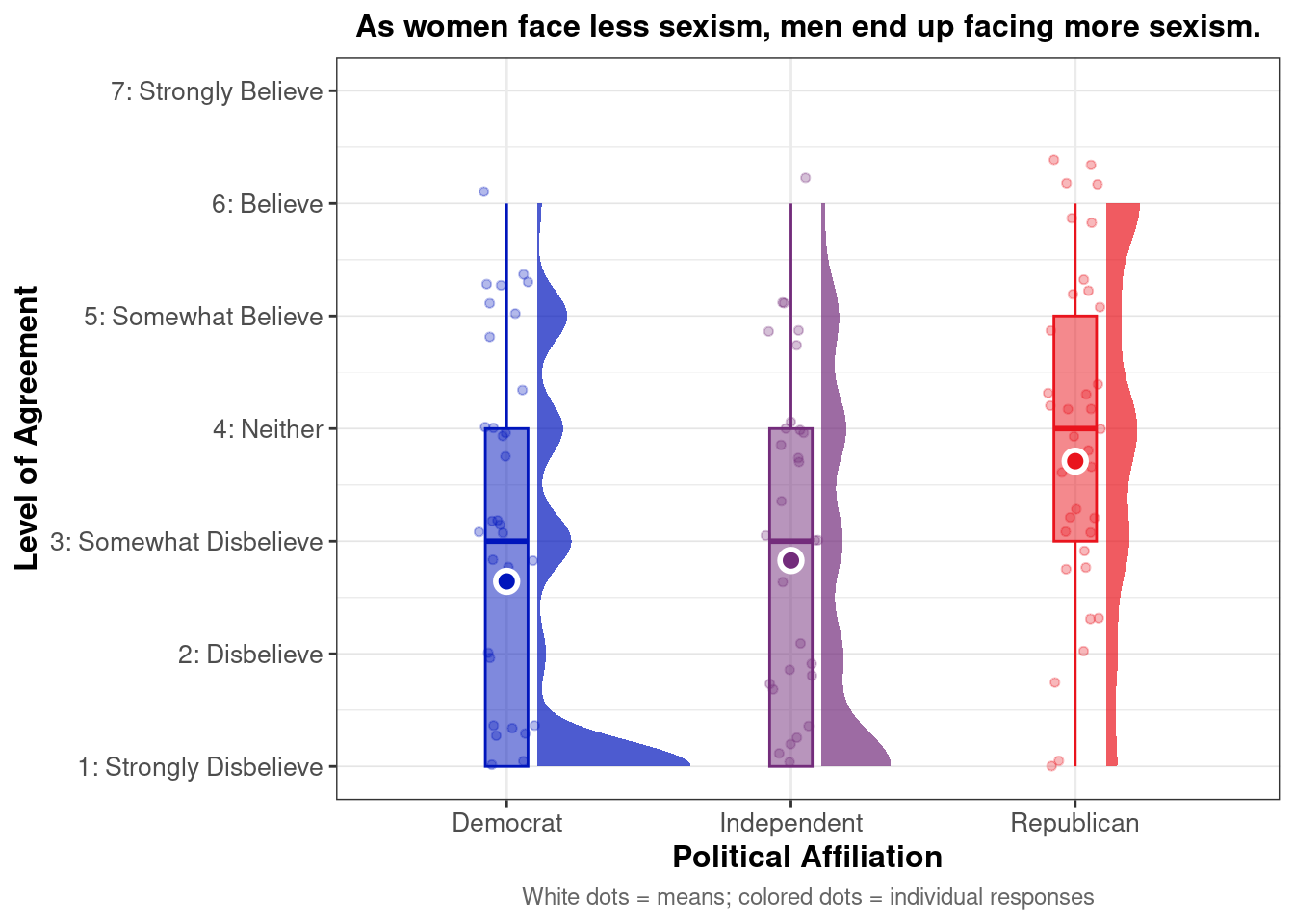
This raincloud plot shows that mean agreement with the zero-sum belief (indicated by white dots) varies by political affiliation. Among the three groups, Republican exhibit higher average agreement with the statement “As women face less sexism, men end up facing more sexism.”

The distribution (via density and individual dots) reveals different patterns across groups. Republicans show a relatively spread distribution with responses concentrated in the moderate-to-high range (3-6) and some clustering around the mean. Independents display a more concentrated distribution around the lower-moderate range with their density peaked around 2-4. Democrats show the most pronounced leftward skew with strong clustering in the low agreement range (1-3) and a long tail extending toward higher values, indicating most Democrats disagree with this zero-sum perspective on gender discrimination.

In [52]:

shapiro_zerosum4 <- select_data %>%
  group_by(RACIALIDENTITY.4) %>%
  summarise(p = shapiro.test(ZEROSUM_4)$p.value)


kable(
  shapiro_zerosum4,
  caption = "Table 31. Shapiro–Wilk Normality Test for ZEROSUM_4 by Racial Identity",
  digits = 4,
  booktabs = TRUE
)

Table 31. Shapiro–Wilk Normality Test for ZEROSUM_4 by Racial Identity

RACIALIDENTITY.4	p
Asian	0.0075
Black	0.0028
Mixed/Other	0.0580
White	0.0001

In [53]:

library(tibble)
library(rempsyc)

kw.ZEROSUM_4.party <- kruskal.test(ZEROSUM_4 ~ POLITICALPARTY, data = select_data)

kw_table <- tibble(
  Predictor = c("POLITICALPARTY"),
  df = c(length(unique(select_data$POLITICALPARTY)) - 1),
  `Chi-squared` = c(round(kw.ZEROSUM_4.party$statistic, 2)),
  p = c(round(kw.ZEROSUM_4.party$p.value, 3))
)

if (knitr::is_html_output()) {
  kw_table %>%
    knitr::kable(
      digits = 3,
      escape = TRUE,
      format = "html",
      caption = "Table 32. Kruskal-Wallis Test Results for ZEROSUM_4"
    ) %>%
    kableExtra::kable_styling(bootstrap_options = c("striped", "hover", "condensed")) %>%
    kableExtra::row_spec(
      which(kw_table$p < 0.05),
      background = "gray"
    )
} else if (knitr::is_latex_output()) {
  kw_table %>%
    knitr::kable(
      digits = 3,
      escape = TRUE,
      format = "latex",
      longtable = TRUE,
      caption = "Kruskal-Wallis Test Results for ZEROSUM\\_4"
    ) %>%
    kableExtra::kable_styling(full_width = FALSE, position = "left") %>%
    kableExtra::row_spec(
      which(kw_table$p < 0.05),
      background = "gray!20"
    )
}

Table 32. Kruskal-Wallis Test Results for ZEROSUM_4

Predictor	df	Chi-squared	p
POLITICALPARTY	2	9.06	0.011

There was significant difference in ZEROSUM_4 scores across political party groups, Kruskal-Wallis χ²(2) = 9.06, p = 0.0108.

Minorities vs. Whites

Do zero-sum beliefs regarding racial discrimination (minorities and whites) differ by racial/ethnic identity and political party affiliation?

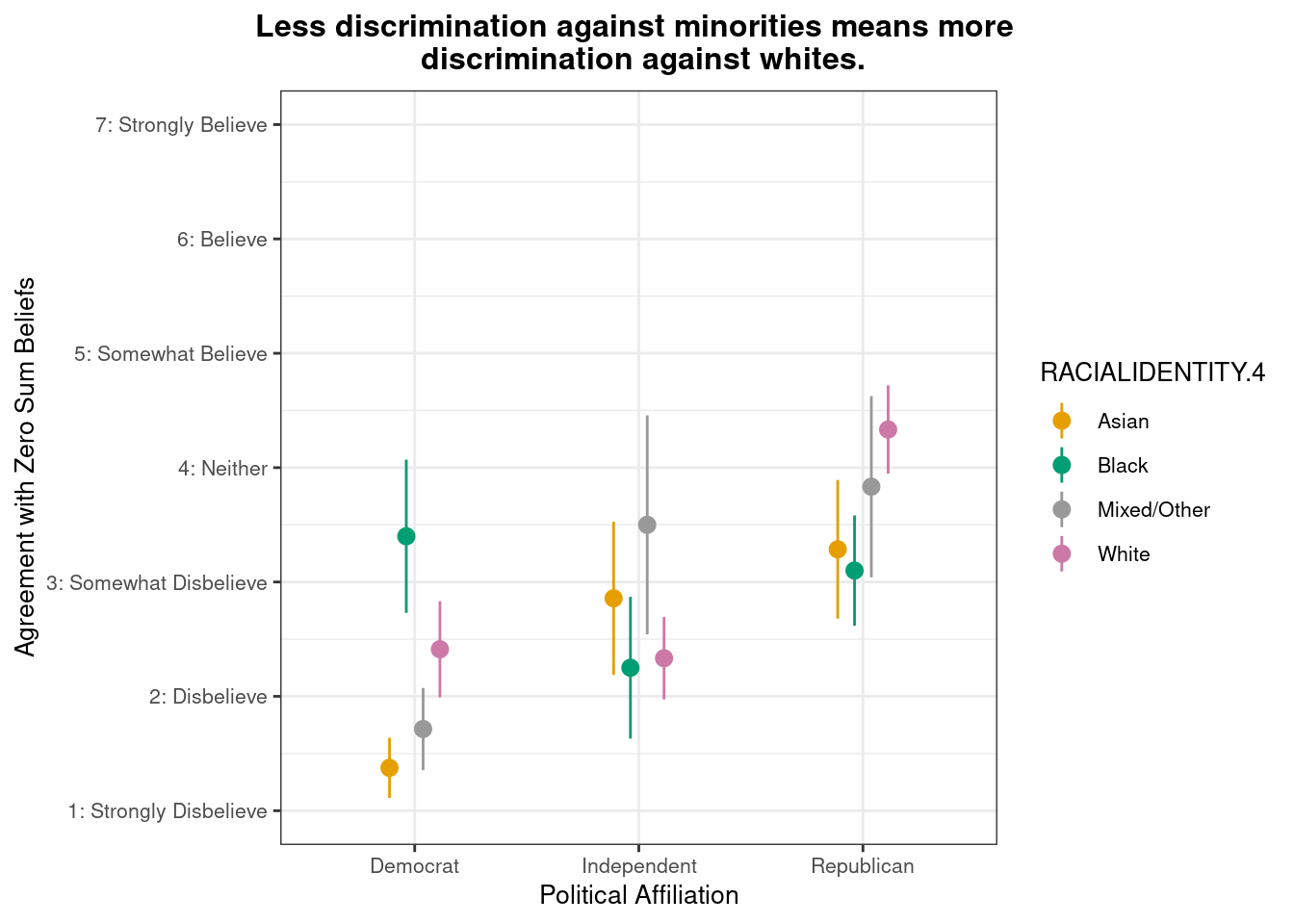
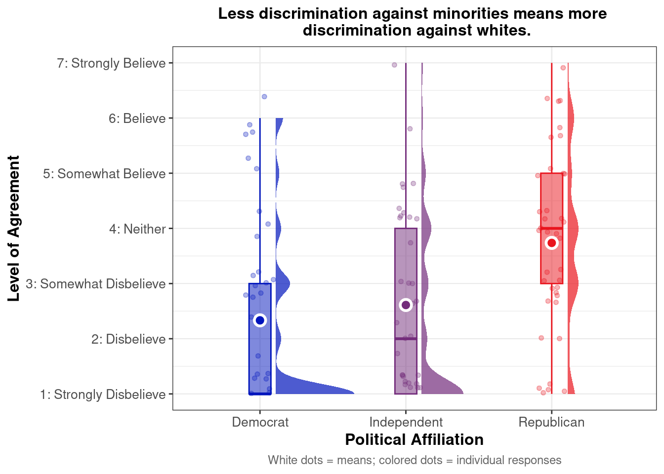
Below we present descriptive statistics and visualizations for ZEROSUM_5 (“Less discrimination against minorities means more discrimination against whites.”), examining how responses vary across racial identity and political affiliation.

In [54]:

library(dplyr)
group_stats_5 <- select_data %>%
  group_by(POLITICALPARTY, RACIALIDENTITY.4) %>%
  summarise(
    mean_ZEROSUM_5 = mean(ZEROSUM_5, na.rm = TRUE),
    se = sd(ZEROSUM_5, na.rm = TRUE) / sqrt(n()),
    .groups = 'drop'
  )

# Check the structure
#str(group_stats_5)

In [55]:

head(group_stats_5)

# A tibble: 6 × 4
  POLITICALPARTY RACIALIDENTITY.4 mean_ZEROSUM_5    se
  <chr>          <chr>                     <dbl> <dbl>
1 Democrat       Asian                      1.38 0.263
2 Democrat       Black                      3.4  0.670
3 Democrat       Mixed/Other                1.71 0.360
4 Democrat       White                      2.41 0.421
5 Independent    Asian                      2.86 0.670
6 Independent    Black                      2.25 0.620

In [56]:

# Define the zesty_four palette
zesty_four <- c("#E69F00", "#009E73", "#999999", "#CC79A7") 

# Create the plot with pointrange
plot.zerosum5 <- ggplot(group_stats_5, aes(POLITICALPARTY, mean_ZEROSUM_5)) +
  geom_pointrange(aes(color = RACIALIDENTITY.4, 
                      ymin = mean_ZEROSUM_5 - se,  # Use standard error instead of sd
                      ymax = mean_ZEROSUM_5 + se), # Use standard error instead of sd
                  position = position_dodge(0.3)) +
  theme_bw() +
  labs(title = "Less discrimination against minorities means more \n discrimination against whites.",
       x = "Political Affiliation",
       y = "Agreement with Zero Sum Beliefs",
       color = "RACIALIDENTITY.4") + 
  theme(
    plot.title = element_text(size = 12, face = "bold", hjust = 0.5),
    axis.title = element_text(size = 10),
    axis.text = element_text(size = 8),
    legend.title = element_text(size = 10),
    legend.text = element_text(size = 8)
  ) +
  scale_y_continuous(
    breaks = 1:7,
    labels = c("1: Strongly Disbelieve", 
               "2: Disbelieve", 
               "3: Somewhat Disbelieve", 
               "4: Neither", 
               "5: Somewhat Believe", 
               "6: Believe", 
               "7: Strongly Believe"),
    limits = c(1, 7)  # Set the y-axis limits to match the scale
  )+
  scale_color_manual(values = zesty_four)

# Print and save the plots
print(plot.zerosum5)

ggsave("plots/plot5:minorities-whites.png", 
       plot = plot.zerosum5, 
       width = 10, 
       height = 8, 
       dpi = 300)

This pointrange plot shows that White respondents exhibit higher agreement with the belief that “Less discrimination against minorities means more discrimination against whites.” among Republicans. Among political groups, Republicans show the highest overall agreement, while Democrats (particularly Asian and Mixed/Other respondents) show the lowest agreement. The pattern highlights how both political affiliation and racial identity intersect to shape zero-sum beliefs about racial discrimination.

In [57]:

# ZEROSUM_5 average score with 95% CI
group_stats_5_avg <- select_data %>%
  group_by(POLITICALPARTY) %>%
  summarise(
    mean_ZEROSUM_5 = mean(ZEROSUM_5, na.rm = TRUE),
    se = sd(ZEROSUM_5, na.rm = TRUE) / sqrt(n()),
    n = n(),
    .groups = 'drop'
  ) %>%
  mutate(
    # Calculate 95% confidence interval using t-distribution
    t_value = qt(0.975, df = n - 1),  # 95% CI, two-tailed
    ci_lower = mean_ZEROSUM_5 - t_value * se,
    ci_upper = mean_ZEROSUM_5 + t_value * se
  )

Do zero-sum beliefs regarding racial discrimination (minorities and whites) differ by political party affiliation?

In [58]:

plot.zerosum5_raincloud <- select_data %>%
  filter(!is.na(ZEROSUM_5), !is.na(POLITICALPARTY)) %>%
  ggplot(aes(x = POLITICALPARTY, y = ZEROSUM_5, fill = POLITICALPARTY, color = POLITICALPARTY)) +
  stat_halfeye(
    adjust = 0.5,
    width = 0.6,
    .width = 0,
    justification = -0.2,
    point_colour = NA,
    alpha = 0.7
  ) +
   geom_boxplot(
    width = 0.15,
    outlier.shape = NA,
    alpha = 0.5
  ) +
  geom_point(
    size = 1.3,
    alpha = 0.3,
    position = position_jitter(
      seed = 1, width = 0.1
    )
  ) +
  stat_summary(
    fun = mean,
    geom = "point",
    size = 3,
    color = "white",
    stroke = 1.5,
    shape = 21
  ) +
  scale_fill_manual(values = party_colors) +
  scale_color_manual(values = party_colors) +
  theme_bw() +
  labs(
    title = "Less discrimination against minorities means more \n discrimination against whites.",
    x = "Political Affiliation",
    y = "Level of Agreement",
    caption = "White dots = means; colored dots = individual responses"
  ) +
  theme(
    plot.title = element_text(size = 12, face = "bold", hjust = 0.5),
    plot.caption = element_text(size = 9, color = "gray40", hjust = 0.5),
    axis.title = element_text(size = 12, face = "bold"),
    axis.text = element_text(size = 10),
    legend.position = "none",
    panel.grid.major.y = element_line(color = "gray90", linewidth = 0.3)  # Fixed
  ) +
  scale_y_continuous(
    breaks = 1:7,
    labels = c("1: Strongly Disbelieve", 
               "2: Disbelieve", 
               "3: Somewhat Disbelieve", 
               "4: Neither", 
               "5: Somewhat Believe", 
               "6: Believe", 
               "7: Strongly Believe"),
    limits = c(1, 7) 
  )
plot.zerosum5_raincloud

Warning: Removed 19 rows containing missing values or values outside the scale range
(`geom_point()`).

This raincloud plot shows that mean agreement with the zero-sum belief (indicated by white dots) varies by political affiliation. Among the three groups, Republican exhibit higher average agreement with the statement “Less discrimination against minorities means more discrimination against whites.” The distribution (via density and individual dots) reveals different patterns across groups. Republicans show a broader distribution with notable density across moderate-to-high agreement levels (3-6), indicating more varied responses within the party. Independents display a relatively concentrated distribution around the lower-moderate range with their density peaked around 1-4. Democrats show strong leftward skew with pronounced clustering in the low agreement range (1-3) and a steep drop-off at higher values, indicating most Democrats reject this zero-sum perspective on racial discrimination.

In [59]:

shapiro_zerosum5 <- select_data %>%
  group_by(RACIALIDENTITY.4) %>%
  summarise(p = shapiro.test(ZEROSUM_5)$p.value)

kable(
  shapiro_zerosum5,
  caption = "Table 33. Shapiro–Wilk Normality Test for ZEROSUM_5 by Racial Identity",
  digits = 4,
  booktabs = TRUE
)

Table 33. Shapiro–Wilk Normality Test for ZEROSUM_5 by Racial Identity

RACIALIDENTITY.4	p
Asian	0.0016
Black	0.0012
Mixed/Other	0.0121
White	0.0002

In [60]:

library(tibble)
library(rempsyc)

kw.ZEROSUM_5.party <- kruskal.test(ZEROSUM_5 ~ POLITICALPARTY, data = select_data)

kw_table <- tibble(
  Predictor = c("POLITICALPARTY"),
  df = c(length(unique(select_data$POLITICALPARTY)) - 1),
  `Chi-squared` = c(round(kw.ZEROSUM_5.party$statistic, 2)),
  p = c(round(kw.ZEROSUM_5.party$p.value, 5))
)

if (knitr::is_html_output()) {
  kw_table %>%
    knitr::kable(
      digits = 5,
      escape = TRUE,
      format = "html",
      caption = "Table 34. Kruskal-Wallis Test Results for ZEROSUM_5"
    ) %>%
    kableExtra::kable_styling(bootstrap_options = c("striped", "hover", "condensed")) %>%
    kableExtra::row_spec(
      which(kw_table$p < 0.05),
      background = "gray"
    )
} else if (knitr::is_latex_output()) {
  kw_table %>%
    knitr::kable(
      digits = 5,
      escape = TRUE,
      format = "latex",
      longtable = TRUE,
      caption = "Kruskal-Wallis Test Results for ZEROSUM\\_5"
    ) %>%
    kableExtra::kable_styling(full_width = FALSE, position = "left") %>%
    kableExtra::row_spec(
      which(kw_table$p < 0.05),
      background = "gray!20"
    )
}

Table 34. Kruskal-Wallis Test Results for ZEROSUM_5

Predictor	df	Chi-squared	p
POLITICALPARTY	2	14.82	0.00061

There was significant difference in ZEROSUM_5 scores across political party groups, Kruskal-Wallis χ²(2) = 14.82, p = 6.06^{-4}.

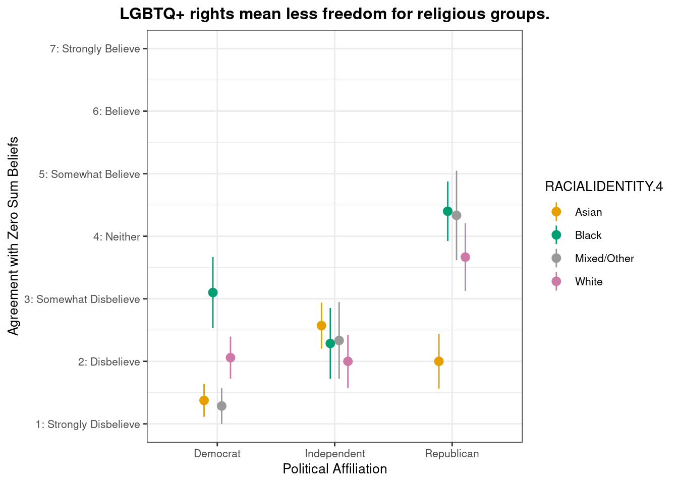
Transgender vs. Cisgender

Do zero-sum beliefs regarding gender identity (transgender and cisgender) differ by racial/ethnic identity and political party affiliation?

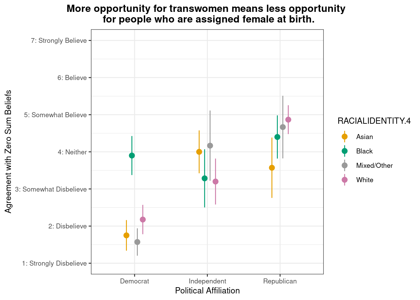
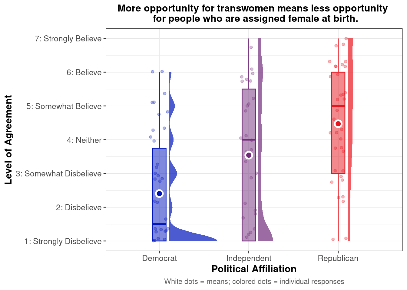
Below we present descriptive statistics and visualizations for ZEROSUM_6 (“More opportunity for transwomen means less opportunity for people who are assigned female at birth.”), examining how responses vary across racial identity and political affiliation.

In [61]:

library(dplyr)
group_stats_6 <- select_data %>%
  group_by(POLITICALPARTY, RACIALIDENTITY.4) %>%
  summarise(
    mean_ZEROSUM_6 = mean(ZEROSUM_6, na.rm = TRUE),
    se = sd(ZEROSUM_6, na.rm = TRUE) / sqrt(n()),
    .groups = 'drop'
  )

# Check the structure
#str(group_stats_6)

In [62]:

head(group_stats_6)

# A tibble: 6 × 4
  POLITICALPARTY RACIALIDENTITY.4 mean_ZEROSUM_6    se
  <chr>          <chr>                     <dbl> <dbl>
1 Democrat       Asian                      1.75 0.412
2 Democrat       Black                      3.9  0.526
3 Democrat       Mixed/Other                1.57 0.369
4 Democrat       White                      2.18 0.395
5 Independent    Asian                      4    0.577
6 Independent    Black                      3.29 0.783

In [63]:

# Define the zesty_four palette
zesty_four <- c("#E69F00", "#009E73", "#999999", "#CC79A7") 

# Create the plot with pointrange
plot.zerosum6 <- ggplot(group_stats_6, aes(POLITICALPARTY, mean_ZEROSUM_6)) +
  geom_pointrange(aes(color = RACIALIDENTITY.4, 
                      ymin = mean_ZEROSUM_6 - se,  # Use standard error instead of sd
                      ymax = mean_ZEROSUM_6 + se), # Use standard error instead of sd
                  position = position_dodge(0.3)) +
  theme_bw() +
  labs(title = "More opportunity for transwomen means less opportunity \n for people who are assigned female at birth.",
       x = "Political Affiliation",
       y = "Agreement with Zero Sum Beliefs",
       color = "RACIALIDENTITY.4") + 
  theme(
    plot.title = element_text(size = 12, face = "bold", hjust = 0.5),
    axis.title = element_text(size = 10),
    axis.text = element_text(size = 8),
    legend.title = element_text(size = 10),
    legend.text = element_text(size = 8)
  ) +
  scale_y_continuous(
    breaks = 1:7,
    labels = c("1: Strongly Disbelieve", 
               "2: Disbelieve", 
               "3: Somewhat Disbelieve", 
               "4: Neither", 
               "5: Somewhat Believe", 
               "6: Believe", 
               "7: Strongly Believe"),
    limits = c(1, 7)  # Set the y-axis limits to match the scale
  )+
  scale_color_manual(values = zesty_four)

# Print and save the plots
print(plot.zerosum6)

ggsave("plots/plot6:trans-cis.png", 
       plot = plot.zerosum6, 
       width = 10, 
       height = 8, 
       dpi = 300)

This pointrange plot shows that White respondents exhibit higher agreement with the belief that “More opportunity for transwomen means less opportunity for people who are assigned female at birth.” among Republicans. Among political groups, Republicans show the highest overall agreement, while Democrats (particularly Asian and Mixed/Other respondents) show the lowest agreement. The pattern highlights how both political affiliation and racial identity intersect to shape zero-sum beliefs about transgender rights and opportunities.

In [64]:

# ZEROSUM_6 average score with 95% CI
group_stats_6_avg <- select_data %>%
  group_by(POLITICALPARTY) %>%
  summarise(
    mean_ZEROSUM_6 = mean(ZEROSUM_6, na.rm = TRUE),
    se = sd(ZEROSUM_6, na.rm = TRUE) / sqrt(n()),
    n = n(),
    .groups = 'drop'
  ) %>%
  mutate(
    # Calculate 95% confidence interval using t-distribution
    t_value = qt(0.975, df = n - 1),  # 95% CI, two-tailed
    ci_lower = mean_ZEROSUM_6 - t_value * se,
    ci_upper = mean_ZEROSUM_6 + t_value * se
  )

Do zero-sum beliefs regarding gender identity (transgender and cisgender) differ by political party affiliation?

In [65]:

plot.zerosum6_raincloud <- select_data %>%
  filter(!is.na(ZEROSUM_6), !is.na(POLITICALPARTY)) %>%
  ggplot(aes(x = POLITICALPARTY, y = ZEROSUM_6, fill = POLITICALPARTY, color = POLITICALPARTY)) +
  stat_halfeye(
    adjust = 0.5,
    width = 0.6,
    .width = 0,
    justification = -0.2,
    point_colour = NA,
    alpha = 0.7
  ) +
   geom_boxplot(
    width = 0.15,
    outlier.shape = NA,
    alpha = 0.5
  ) +
  geom_point(
    size = 1.3,
    alpha = 0.3,
    position = position_jitter(
      seed = 1, width = 0.1
    )
  ) +
  stat_summary(
    fun = mean,
    geom = "point",
    size = 3,
    color = "white",
    stroke = 1.5,
    shape = 21
  ) +
  scale_fill_manual(values = party_colors) +
  scale_color_manual(values = party_colors) +
  theme_bw() +
  labs(
    title = "More opportunity for transwomen means less opportunity \n for people who are assigned female at birth.",
    x = "Political Affiliation",
    y = "Level of Agreement",
    caption = "White dots = means; colored dots = individual responses"
  ) +
  theme(
    plot.title = element_text(size = 12, face = "bold", hjust = 0.5),
    plot.caption = element_text(size = 9, color = "gray40", hjust = 0.5),
    axis.title = element_text(size = 12, face = "bold"),
    axis.text = element_text(size = 10),
    legend.position = "none",
    panel.grid.major.y = element_line(color = "gray90", linewidth = 0.3)  # Fixed
  ) +
  scale_y_continuous(
    breaks = 1:7,
    labels = c("1: Strongly Disbelieve", 
               "2: Disbelieve", 
               "3: Somewhat Disbelieve", 
               "4: Neither", 
               "5: Somewhat Believe", 
               "6: Believe", 
               "7: Strongly Believe"),
    limits = c(1, 7) 
  )
plot.zerosum6_raincloud

Warning: Removed 22 rows containing missing values or values outside the scale range
(`geom_point()`).

This raincloud plot shows that mean agreement with the zero-sum belief (indicated by white dots) varies by political affiliation. Among the three groups, Republican exhibit higher average agreement with the statement “More opportunity for transwomen means less opportunity for people who are assigned female at birth.”

The distribution (via density and individual dots) reveals different patterns across groups. Republicans show a relatively concentrated distribution around moderate-to-high agreement levels (3-6) with some spread toward the extremes. Independents display a broad distribution with responses spanning from low to high agreement but concentrated in the moderate range (2-6). Democrats show strong leftward skew with pronounced clustering in the low agreement range (1-3) and a steep drop-off at higher values, indicating most Democrats reject this zero-sum perspective on transgender rights and opportunities.

In [66]:

shapiro_zerosum6 <- select_data %>%
  group_by(RACIALIDENTITY.4) %>%
  summarise(p = shapiro.test(ZEROSUM_6)$p.value)

kable(
  shapiro_zerosum6,
  caption = "Table 35. Shapiro–Wilk Normality Test for ZEROSUM_6 by Racial Identity",
  digits = 5,
  booktabs = TRUE
)

Table 35. Shapiro–Wilk Normality Test for ZEROSUM_6 by Racial Identity

RACIALIDENTITY.4	p
Asian	0.02164
Black	0.03789
Mixed/Other	0.01372
White	0.00003

In [67]:

library(tibble)
library(rempsyc)

kw.ZEROSUM_6.party <- kruskal.test(ZEROSUM_6 ~ POLITICALPARTY, data = select_data)

kw_table <- tibble(
  Predictor = c("POLITICALPARTY"),
  df = c(length(unique(select_data$POLITICALPARTY)) - 1),
  `Chi-squared` = c(round(kw.ZEROSUM_6.party$statistic, 2)),
  p = c(round(kw.ZEROSUM_6.party$p.value, 5))
)

if (knitr::is_html_output()) {
  kw_table %>%
    knitr::kable(
      digits = 5,
      escape = TRUE,
      format = "html",
      caption = "Table 36. Kruskal-Wallis Test Results for ZEROSUM_6"
    ) %>%
    kableExtra::kable_styling(bootstrap_options = c("striped", "hover", "condensed")) %>%
    kableExtra::row_spec(
      which(kw_table$p < 0.05),
      background = "gray"
    )
} else if (knitr::is_latex_output()) {
  kw_table %>%
    knitr::kable(
      digits = 5,
      escape = TRUE,
      format = "latex",
      longtable = TRUE,
      caption = "Kruskal-Wallis Test Results for ZEROSUM\\_6"
    ) %>%
    kableExtra::kable_styling(full_width = FALSE, position = "left") %>%
    kableExtra::row_spec(
      which(kw_table$p < 0.05),
      background = "gray!20"
    )
}

Table 36. Kruskal-Wallis Test Results for ZEROSUM_6

Predictor	df	Chi-squared	p
POLITICALPARTY	2	20.98	3e-05

There was significant difference in ZEROSUM_6 scores across political party groups, Kruskal-Wallis χ²(2) = 20.98, p = 2.79^{-5}.

Undocumented vs. Citizens

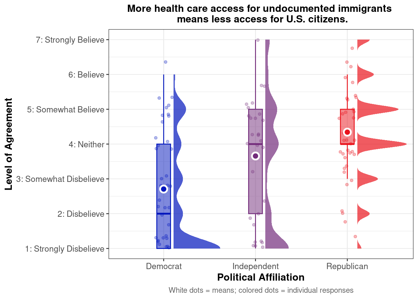
Do zero-sum beliefs about healthcare access—specifically, that undocumented immigration reduces access for U.S. citizens—differ by racial/ethnic identity and political affiliation?

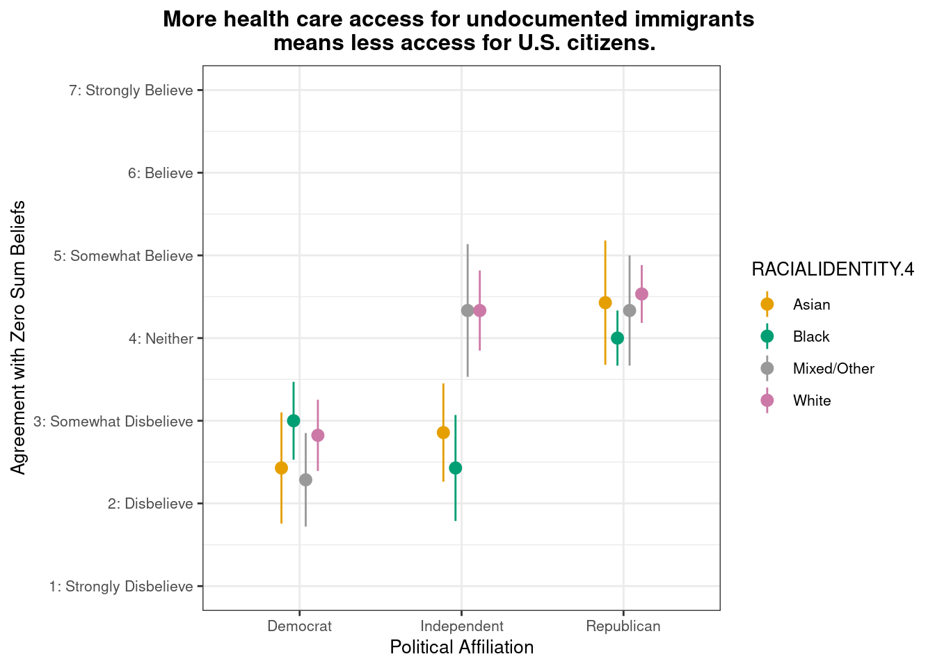
Below we present descriptive statistics and visualizations for ZEROSUM_7 (“More health care access for undocumented immigrants means less access for U.S. citizens.”), examining how responses vary across racial identity and political affiliation.

In [68]:

library(dplyr)
group_stats_7 <- select_data %>%
  group_by(POLITICALPARTY, RACIALIDENTITY.4) %>%
  summarise(
    mean_ZEROSUM_7 = mean(ZEROSUM_7, na.rm = TRUE),
    se = sd(ZEROSUM_7, na.rm = TRUE) / sqrt(n()),
    .groups = 'drop'
  )

# Check the structure
#str(group_stats_7)

In [69]:

head(group_stats_7)

# A tibble: 6 × 4
  POLITICALPARTY RACIALIDENTITY.4 mean_ZEROSUM_7    se
  <chr>          <chr>                     <dbl> <dbl>
1 Democrat       Asian                      2.43 0.673
2 Democrat       Black                      3    0.471
3 Democrat       Mixed/Other                2.29 0.565
4 Democrat       White                      2.82 0.431
5 Independent    Asian                      2.86 0.595
6 Independent    Black                      2.43 0.641

In [70]:

# Define the zesty_four palette
zesty_four <- c("#E69F00", "#009E73", "#999999", "#CC79A7") 

# Create the plot with pointrange
plot.zerosum7 <- ggplot(group_stats_7, aes(POLITICALPARTY, mean_ZEROSUM_7)) +
  geom_pointrange(aes(color = RACIALIDENTITY.4, 
                      ymin = mean_ZEROSUM_7 - se,  # Use standard error instead of sd
                      ymax = mean_ZEROSUM_7 + se), # Use standard error instead of sd
                  position = position_dodge(0.3)) +
  theme_bw() +
  labs(title = "More health care access for undocumented immigrants \n means less access for U.S. citizens.",
       x = "Political Affiliation",
       y = "Agreement with Zero Sum Beliefs",
       color = "RACIALIDENTITY.4") + 
  theme(
    plot.title = element_text(size = 12, face = "bold", hjust = 0.5),
    axis.title = element_text(size = 10),
    axis.text = element_text(size = 8),
    legend.title = element_text(size = 10),
    legend.text = element_text(size = 8)
  ) +
  scale_y_continuous(
    breaks = 1:7,
    labels = c("1: Strongly Disbelieve", 
               "2: Disbelieve", 
               "3: Somewhat Disbelieve", 
               "4: Neither", 
               "5: Somewhat Believe", 
               "6: Believe", 
               "7: Strongly Believe"),
    limits = c(1, 7)  # Set the y-axis limits to match the scale
  )+
  scale_color_manual(values = zesty_four)

# Print and save the plots
print(plot.zerosum7)

ggsave("plots/plot7:undoc-citizens.png", 
       plot = plot.zerosum7, 
       width = 10, 
       height = 8, 
       dpi = 300)

This pointrange plot shows that Asian respondents exhibit higher agreement with the belief that “More health care access for undocumented immigrants means less access for U.S. citizens.” among Republicans. Among political groups, Republicans show the highest overall agreement, while Democrats (particularly Asian and Mixed/Other respondents) show the lowest agreement. This pattern highlights that political affiliation creates a greater divide in zero-sum beliefs about health care resources within each political group than does racial identity.

In [71]:

# ZEROSUM_7 average score with 95% CI
group_stats_7_avg <- select_data %>%
  group_by(POLITICALPARTY) %>%
  summarise(
    mean_ZEROSUM_7 = mean(ZEROSUM_7, na.rm = TRUE),
    se = sd(ZEROSUM_7, na.rm = TRUE) / sqrt(n()),
    n = n(),
    .groups = 'drop'
  ) %>%
  mutate(
    # Calculate 95% confidence interval using t-distribution
    t_value = qt(0.975, df = n - 1),  # 95% CI, two-tailed
    ci_lower = mean_ZEROSUM_7 - t_value * se,
    ci_upper = mean_ZEROSUM_7 + t_value * se
  )

Do zero-sum beliefs about healthcare access—specifically, that undocumented immigration reduces access for U.S. citizens—differ by political affiliation?

In [72]:

plot.zerosum7_raincloud <- select_data %>%
  filter(!is.na(ZEROSUM_7), !is.na(POLITICALPARTY)) %>%
  ggplot(aes(x = POLITICALPARTY, y = ZEROSUM_7, fill = POLITICALPARTY, color = POLITICALPARTY)) +
  stat_halfeye(
    adjust = 0.5,
    width = 0.6,
    .width = 0,
    justification = -0.2,
    point_colour = NA,
    alpha = 0.7
  ) +
   geom_boxplot(
    width = 0.15,
    outlier.shape = NA,
    alpha = 0.5
  ) +
  geom_point(
    size = 1.3,
    alpha = 0.3,
    position = position_jitter(
      seed = 1, width = 0.1
    )
  ) +
  stat_summary(
    fun = mean,
    geom = "point",
    size = 3,
    color = "white",
    stroke = 1.5,
    shape = 21
  ) +
  scale_fill_manual(values = party_colors) +
  scale_color_manual(values = party_colors) +
  theme_bw() +
  labs(
    title = "More health care access for undocumented immigrants \n means less access for U.S. citizens.",
    x = "Political Affiliation",
    y = "Level of Agreement",
    caption = "White dots = means; colored dots = individual responses"
  ) +
  theme(
    plot.title = element_text(size = 12, face = "bold", hjust = 0.5),
    plot.caption = element_text(size = 9, color = "gray40", hjust = 0.5),
    axis.title = element_text(size = 12, face = "bold"),
    axis.text = element_text(size = 10),
    legend.position = "none",
    panel.grid.major.y = element_line(color = "gray90", linewidth = 0.3)  # Fixed
  ) +
  scale_y_continuous(
    breaks = 1:7,
    labels = c("1: Strongly Disbelieve", 
               "2: Disbelieve", 
               "3: Somewhat Disbelieve", 
               "4: Neither", 
               "5: Somewhat Believe", 
               "6: Believe", 
               "7: Strongly Believe"),
    limits = c(1, 7) 
  )
plot.zerosum7_raincloud

Warning: Removed 11 rows containing missing values or values outside the scale range
(`geom_point()`).

This raincloud plot shows that mean agreement with the zero-sum belief (indicated by white dots) varies by political affiliation. Among the three groups, Republican exhibit higher average agreement with the statement “More health care access for undocumented immigrants means less access for U.S. citizens.” The distribution (via density and individual dots) reveals different patterns across groups. Republicans show a relatively concentrated distribution around moderate-to-high agreement levels (4-6) with their density peaked around the mean. Independents display a broader, more spread distribution across the full range with notable presence from low to high agreement levels. Democrats show strong leftward skew with pronounced clustering in the low agreement range (1-3) and a steep drop-off at higher values, indicating most Democrats reject this zero-sum perspective on healthcare access.

In [73]:

shapiro_zerosum7 <- select_data %>%
  group_by(RACIALIDENTITY.4) %>%
  summarise(p = shapiro.test(ZEROSUM_7)$p.value)

kable(
  shapiro_zerosum7,
  caption = "Table 37. Shapiro–Wilk Normality Test for ZEROSUM_7 by Racial Identity",
  digits = 5,
  booktabs = TRUE
)

Table 37. Shapiro–Wilk Normality Test for ZEROSUM_7 by Racial Identity

RACIALIDENTITY.4	p
Asian	0.03876
Black	0.00150
Mixed/Other	0.10149
White	0.00292

In [74]:

library(tibble)
library(rempsyc)

kw.ZEROSUM_7.party <- kruskal.test(ZEROSUM_7 ~ POLITICALPARTY, data = select_data)

kw_table <- tibble(
  Predictor = c("POLITICALPARTY"),
  df = c(length(unique(select_data$POLITICALPARTY)) - 1),
  `Chi-squared` = c(round(kw.ZEROSUM_7.party$statistic, 2)),
  p = c(round(kw.ZEROSUM_7.party$p.value, 5))
)

if (knitr::is_html_output()) {
  kw_table %>%
    knitr::kable(
      digits = 5,
      escape = TRUE,
      format = "html",
      caption = "Table 38. Kruskal-Wallis Test Results for ZEROSUM_7"
    ) %>%
    kableExtra::kable_styling(bootstrap_options = c("striped", "hover", "condensed")) %>%
    kableExtra::row_spec(
      which(kw_table$p < 0.05),
      background = "gray"
    )
} else if (knitr::is_latex_output()) {
  kw_table %>%
    knitr::kable(
      digits = 5,
      escape = TRUE,
      format = "latex",
      longtable = TRUE,
      caption = "Kruskal-Wallis Test Results for ZEROSUM\\_7"
    ) %>%
    kableExtra::kable_styling(full_width = FALSE, position = "left") %>%
    kableExtra::row_spec(
      which(kw_table$p < 0.05),
      background = "gray!20"
    )
}

Table 38. Kruskal-Wallis Test Results for ZEROSUM_7

Predictor	df	Chi-squared	p
POLITICALPARTY	2	15.35	0.00046

There was significant difference in ZEROSUM_7 scores across political party groups, Kruskal-Wallis χ²(2) = 15.35, p = 4.63^{-4}.

Paywomen vs. men

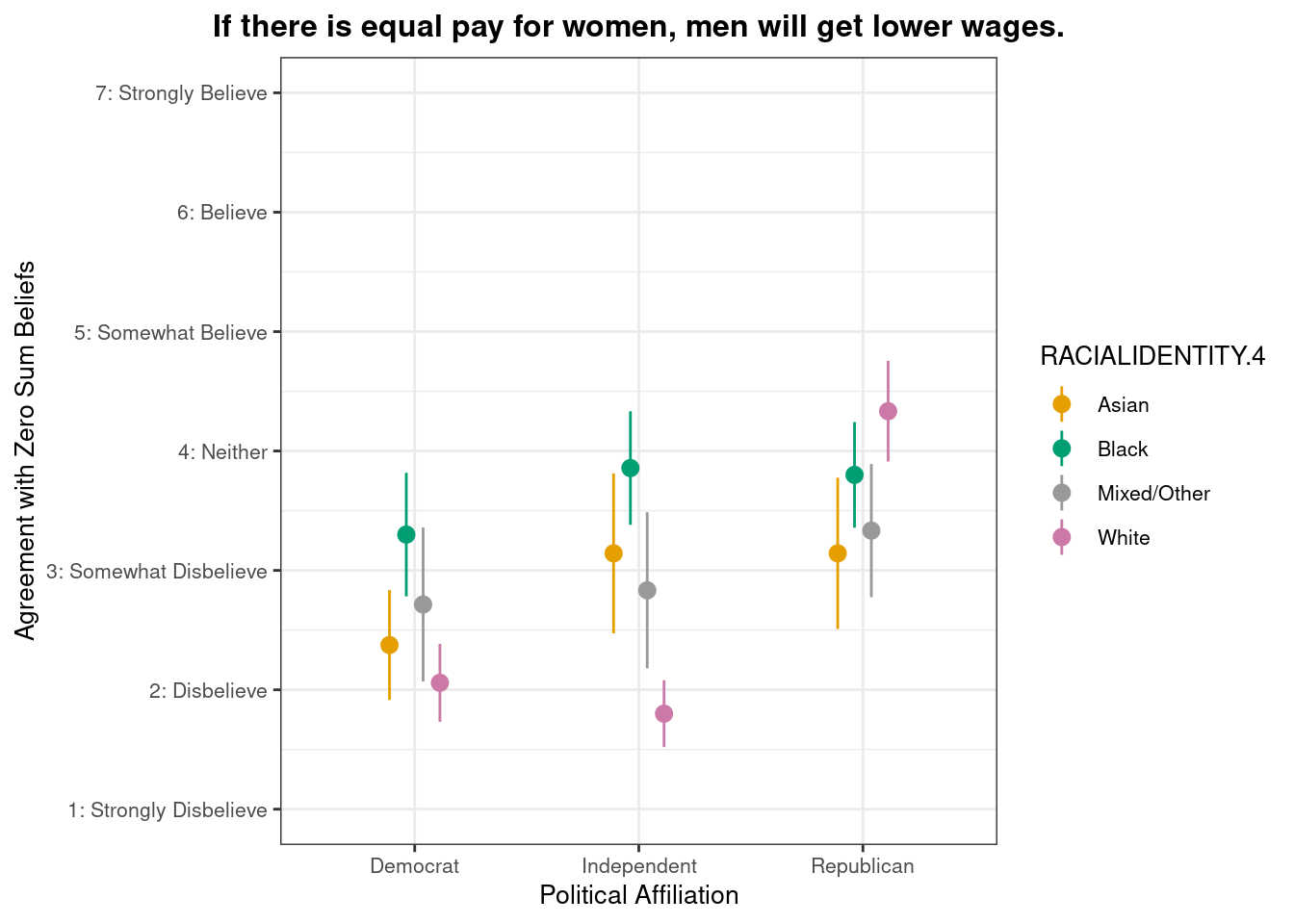
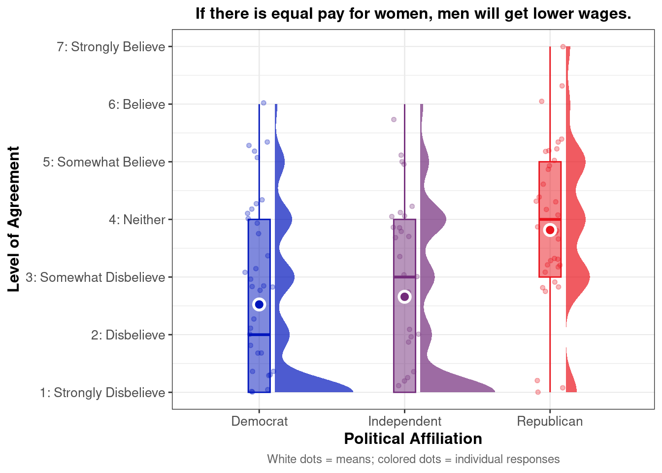
Do zero-sum beliefs regarding gender pay equity differ by racial/ethnic identity and political party affiliation?

Below we present descriptive statistics and visualizations for ZEROSUM_8 (“If there is equal pay for women, men will get lower wages.”), examining how responses vary across racial identity and political affiliation.

In [75]:

library(dplyr)
group_stats_8 <- select_data %>%
  group_by(POLITICALPARTY, RACIALIDENTITY.4) %>%
  summarise(
    mean_ZEROSUM_8 = mean(ZEROSUM_8, na.rm = TRUE),
    se = sd(ZEROSUM_8, na.rm = TRUE) / sqrt(n()),
    .groups = 'drop'
  )

# Check the structure
#str(group_stats_8)

In [76]:

head(group_stats_8)

# A tibble: 6 × 4
  POLITICALPARTY RACIALIDENTITY.4 mean_ZEROSUM_8    se
  <chr>          <chr>                     <dbl> <dbl>
1 Democrat       Asian                      2.38 0.460
2 Democrat       Black                      3.3  0.517
3 Democrat       Mixed/Other                2.71 0.644
4 Democrat       White                      2.06 0.326
5 Independent    Asian                      3.14 0.670
6 Independent    Black                      3.86 0.476

In [77]:

# Define the zesty_four palette
zesty_four <- c("#E69F00", "#009E73", "#999999", "#CC79A7") 

# Create the plot with pointrange
plot.zerosum8 <- ggplot(group_stats_8, aes(POLITICALPARTY, mean_ZEROSUM_8)) +
  geom_pointrange(aes(color = RACIALIDENTITY.4, 
                      ymin = mean_ZEROSUM_8 - se,  # Use standard error instead of sd
                      ymax = mean_ZEROSUM_8 + se), # Use standard error instead of sd
                  position = position_dodge(0.3)) +
  theme_bw() +
  labs(title = "If there is equal pay for women, men will get lower wages.",
       x = "Political Affiliation",
       y = "Agreement with Zero Sum Beliefs",
       color = "RACIALIDENTITY.4") + 
  theme(
    plot.title = element_text(size = 12, face = "bold", hjust = 0.5),
    axis.title = element_text(size = 10),
    axis.text = element_text(size = 8),
    legend.title = element_text(size = 10),
    legend.text = element_text(size = 8)
  ) +
  scale_y_continuous(
    breaks = 1:7,
    labels = c("1: Strongly Disbelieve", 
               "2: Disbelieve", 
               "3: Somewhat Disbelieve", 
               "4: Neither", 
               "5: Somewhat Believe", 
               "6: Believe", 
               "7: Strongly Believe"),
    limits = c(1, 7)  # Set the y-axis limits to match the scale
  )+
  scale_color_manual(values = zesty_four)

# Print and save the plots
print(plot.zerosum8)

ggsave("plots/plot8:paywomen-men.png", 
       plot = plot.zerosum8, 
       width = 10, 
       height = 8, 
       dpi = 300)

This pointrange plot shows that White respondents exhibit higher agreement with the belief that “If there is equal pay for women, men will get lower wages.” among Republicans. Among political groups, Republicans show the highest overall agreement, while Democrats across all racial groups showed lower levels of agreement (2-3 range), with white respondents showing the lowest agreement. This pattern highlights how political affiliation creates major divisions in zero-sum beliefs about gender pay equality, with racial differences more pronounced among Republicans than other political groups.

In [78]:

# ZEROSUM_8 average score with 95% CI
group_stats_8_avg <- select_data %>%
  group_by(POLITICALPARTY) %>%
  summarise(
    mean_ZEROSUM_8 = mean(ZEROSUM_8, na.rm = TRUE),
    se = sd(ZEROSUM_8, na.rm = TRUE) / sqrt(n()),
    n = n(),
    .groups = 'drop'
  ) %>%
  mutate(
    # Calculate 95% confidence interval using t-distribution
    t_value = qt(0.975, df = n - 1),  # 95% CI, two-tailed
    ci_lower = mean_ZEROSUM_8 - t_value * se,
    ci_upper = mean_ZEROSUM_8 + t_value * se
  )

Do zero-sum beliefs regarding gender pay equity differ by political party affiliation?

In [79]:

plot.zerosum8_raincloud <- select_data %>%
  filter(!is.na(ZEROSUM_8), !is.na(POLITICALPARTY)) %>%
  ggplot(aes(x = POLITICALPARTY, y = ZEROSUM_8, fill = POLITICALPARTY, color = POLITICALPARTY)) +
  stat_halfeye(
    adjust = 0.5,
    width = 0.6,
    .width = 0,
    justification = -0.2,
    point_colour = NA,
    alpha = 0.7
  ) +
   geom_boxplot(
    width = 0.15,
    outlier.shape = NA,
    alpha = 0.5
  ) +
  geom_point(
    size = 1.3,
    alpha = 0.3,
    position = position_jitter(
      seed = 1, width = 0.1
    )
  ) +
  stat_summary(
    fun = mean,
    geom = "point",
    size = 3,
    color = "white",
    stroke = 1.5,
    shape = 21
  ) +
  scale_fill_manual(values = party_colors) +
  scale_color_manual(values = party_colors) +
  theme_bw() +
  labs(
    title = "If there is equal pay for women, men will get lower wages.",
    x = "Political Affiliation",
    y = "Level of Agreement",
    caption = "White dots = means; colored dots = individual responses"
  ) +
  theme(
    plot.title = element_text(size = 12, face = "bold", hjust = 0.5),
    plot.caption = element_text(size = 9, color = "gray40", hjust = 0.5),
    axis.title = element_text(size = 12, face = "bold"),
    axis.text = element_text(size = 10),
    legend.position = "none",
    panel.grid.major.y = element_line(color = "gray90", linewidth = 0.3)  # Fixed
  ) +
  scale_y_continuous(
    breaks = 1:7,
    labels = c("1: Strongly Disbelieve", 
               "2: Disbelieve", 
               "3: Somewhat Disbelieve", 
               "4: Neither", 
               "5: Somewhat Believe", 
               "6: Believe", 
               "7: Strongly Believe"),
    limits = c(1, 7) 
  )
plot.zerosum8_raincloud

Warning: Removed 21 rows containing missing values or values outside the scale range
(`geom_point()`).

This raincloud plot shows that mean agreement with the zero-sum belief (indicated by white dots) varies by political affiliation. Among the three groups, Republican exhibit higher average agreement with the statement “If there is equal pay for women, men will get lower wages.” Independents and Democrats show similar mean agreement levels at lower values. The distribution (via density and individual dots) reveals different patterns across groups. Republicans show a relatively concentrated distribution around moderate agreement levels (3-5) with their density peaked around the mean. Both independents and Democrats show very similar distributions, ranging widely across low to moderate levels of agreement (1-5). This suggests that both groups have similar overall skepticism about this zero-sum view of gender pay equality.

In [80]:

shapiro_zerosum8 <- select_data %>%
  group_by(RACIALIDENTITY.4) %>%
  summarise(p = shapiro.test(ZEROSUM_8)$p.value)

kable(
  shapiro_zerosum8,
  caption = "Table 39. Shapiro–Wilk Normality Test for ZEROSUM_8 by Racial Identity",
  digits = 5,
  booktabs = TRUE
)

Table 39. Shapiro–Wilk Normality Test for ZEROSUM_8 by Racial Identity

RACIALIDENTITY.4	p
Asian	0.01744
Black	0.01325
Mixed/Other	0.01982
White	0.00004

In [81]:

library(tibble)
library(rempsyc)

kw.ZEROSUM_8.party <- kruskal.test(ZEROSUM_8 ~ POLITICALPARTY, data = select_data)

kw_table <- tibble(
  Predictor = c("POLITICALPARTY"),
  df = c(length(unique(select_data$POLITICALPARTY)) - 1),
  `Chi-squared` = c(round(kw.ZEROSUM_8.party$statistic, 2)),
  p = c(round(kw.ZEROSUM_8.party$p.value, 5))
)

if (knitr::is_html_output()) {
  kw_table %>%
    knitr::kable(
      digits = 5,
      escape = TRUE,
      format = "html",
      caption = "Table 40. Kruskal-Wallis Test Results for ZEROSUM_8"
    ) %>%
    kableExtra::kable_styling(bootstrap_options = c("striped", "hover", "condensed")) %>%
    kableExtra::row_spec(
      which(kw_table$p < 0.05),
      background = "gray"
    )
} else if (knitr::is_latex_output()) {
  kw_table %>%
    knitr::kable(
      digits = 5,
      escape = TRUE,
      format = "latex",
      longtable = TRUE,
      caption = "Kruskal-Wallis Test Results for ZEROSUM\\_8"
    ) %>%
    kableExtra::kable_styling(full_width = FALSE, position = "left") %>%
    kableExtra::row_spec(
      which(kw_table$p < 0.05),
      background = "gray!20"
    )
}

Table 40. Kruskal-Wallis Test Results for ZEROSUM_8

Predictor	df	Chi-squared	p
POLITICALPARTY	2	13.51	0.00117

There was significant difference in ZEROSUM_8 scores across political party groups, Kruskal-Wallis χ²(2) = 13.51, p = 0.00117.

LGBTQ vs. Religious

Do zero-sum beliefs regarding LGBTQ+ rights and religious freedom differ by racial/ethnic identity and political party affiliation?

Below we present descriptive statistics and visualizations for ZEROSUM_9 (“LGBTQ+ rights mean less freedom for religious groups.”), examining how responses vary across racial identity and political affiliation.

In [82]:

library(dplyr)
group_stats_9 <- select_data %>%
  group_by(POLITICALPARTY, RACIALIDENTITY.4) %>%
  summarise(
    mean_ZEROSUM_9 = mean(ZEROSUM_9, na.rm = TRUE),
    se = sd(ZEROSUM_9, na.rm = TRUE) / sqrt(n()),
    .groups = 'drop'
  )

# Check the structure
#str(group_stats_9)

In [83]:

head(group_stats_9)

# A tibble: 6 × 4
  POLITICALPARTY RACIALIDENTITY.4 mean_ZEROSUM_9    se
  <chr>          <chr>                     <dbl> <dbl>
1 Democrat       Asian                      1.38 0.263
2 Democrat       Black                      3.1  0.567
3 Democrat       Mixed/Other                1.29 0.286
4 Democrat       White                      2.06 0.337
5 Independent    Asian                      2.57 0.369
6 Independent    Black                      2.29 0.567

In [84]:

# Define the zesty_four palette
zesty_four <- c("#E69F00", "#009E73", "#999999", "#CC79A7") 

# Create the plot with pointrange
plot.zerosum9 <- ggplot(group_stats_9, aes(POLITICALPARTY, mean_ZEROSUM_9)) +
  geom_pointrange(aes(color = RACIALIDENTITY.4, 
                      ymin = mean_ZEROSUM_9 - se,  # Use standard error instead of sd
                      ymax = mean_ZEROSUM_9 + se), # Use standard error instead of sd
                  position = position_dodge(0.3)) +
  theme_bw() +
  labs(title = "LGBTQ+ rights mean less freedom for religious groups.",
       x = "Political Affiliation",
       y = "Agreement with Zero Sum Beliefs",
       color = "RACIALIDENTITY.4") + 
  theme(
    plot.title = element_text(size = 12, face = "bold", hjust = 0.5),
    axis.title = element_text(size = 10),
    axis.text = element_text(size = 8),
    legend.title = element_text(size = 10),
    legend.text = element_text(size = 8)
  ) +
  scale_y_continuous(
    breaks = 1:7,
    labels = c("1: Strongly Disbelieve", 
               "2: Disbelieve", 
               "3: Somewhat Disbelieve", 
               "4: Neither", 
               "5: Somewhat Believe", 
               "6: Believe", 
               "7: Strongly Believe"),
    limits = c(1, 7)  # Set the y-axis limits to match the scale
  )+
  scale_color_manual(values = zesty_four)

# Print and save the plots
print(plot.zerosum9)

ggsave("plots/plot9:LGBTQ-religious.png", 
       plot = plot.zerosum9, 
       width = 10, 
       height = 8, 
       dpi = 300)

This pointrange plot shows that Black respondents exhibit higher agreement with the belief that “LGBTQ+ rights mean less freedom for religious groups.” among Republicans. Among political groups, Republicans show the highest overall agreement, while Democrats across all racial groups showed lower levels of agreement (1-2 range), with Mixed/Other and Asian respondents showing the lowest agreement. This pattern captures how political affiliation creates major divisions in zero-sum beliefs about LGBTQ+ and religious rights, with significant racial differences occurring primarily among Republicans.

In [85]:

# ZEROSUM_9 average score with 95% CI
group_stats_9_avg <- select_data %>%
  group_by(POLITICALPARTY) %>%
  summarise(
    mean_ZEROSUM_9 = mean(ZEROSUM_9, na.rm = TRUE),
    se = sd(ZEROSUM_9, na.rm = TRUE) / sqrt(n()),
    n = n(),
    .groups = 'drop'
  ) %>%
  mutate(
    # Calculate 95% confidence interval using t-distribution
    t_value = qt(0.975, df = n - 1),  # 95% CI, two-tailed
    ci_lower = mean_ZEROSUM_9 - t_value * se,
    ci_upper = mean_ZEROSUM_9 + t_value * se
  )

Do zero-sum beliefs regarding LGBTQ+ rights and religious freedom differ by political party affiliation?

In [86]:

plot.zerosum9_raincloud <- select_data %>%
  filter(!is.na(ZEROSUM_9), !is.na(POLITICALPARTY)) %>%
  ggplot(aes(x = POLITICALPARTY, y = ZEROSUM_9, fill = POLITICALPARTY, color = POLITICALPARTY)) +
  stat_halfeye(
    adjust = 0.5,
    width = 0.6,
    .width = 0,
    justification = -0.2,
    point_colour = NA,
    alpha = 0.7
  ) +
   geom_boxplot(
    width = 0.15,
    outlier.shape = NA,
    alpha = 0.5
  ) +
  geom_point(
    size = 1.3,
    alpha = 0.3,
    position = position_jitter(
      seed = 1, width = 0.1
    )
  ) +
  stat_summary(
    fun = mean,
    geom = "point",
    size = 3,
    color = "white",
    stroke = 1.5,
    shape = 21
  ) +
  scale_fill_manual(values = party_colors) +
  scale_color_manual(values = party_colors) +
  theme_bw() +
  labs(
    title = "LGBTQ+ rights mean less freedom for religious groups.",
    x = "Political Affiliation",
    y = "Level of Agreement",
    caption = "White dots = means; colored dots = individual responses"
  ) +
  theme(
    plot.title = element_text(size = 12, face = "bold", hjust = 0.5),
    plot.caption = element_text(size = 9, color = "gray40", hjust = 0.5),
    axis.title = element_text(size = 12, face = "bold"),
    axis.text = element_text(size = 10),
    legend.position = "none",
    panel.grid.major.y = element_line(color = "gray90", linewidth = 0.3)  # Fixed
  ) +
  scale_y_continuous(
    breaks = 1:7,
    labels = c("1: Strongly Disbelieve", 
               "2: Disbelieve", 
               "3: Somewhat Disbelieve", 
               "4: Neither", 
               "5: Somewhat Believe", 
               "6: Believe", 
               "7: Strongly Believe"),
    limits = c(1, 7) 
  )
plot.zerosum9_raincloud

Warning: Removed 27 rows containing missing values or values outside the scale range
(`geom_point()`).

This raincloud plot shows that mean agreement with the zero-sum belief (indicated by white dots) varies by political affiliation. Among the three groups, Republican exhibit higher average agreement with the statement “LGBTQ+ rights mean less freedom for religious groups.” The distribution (via density and individual dots) reveals different patterns across groups. Republicans show a broad distribution with responses spanning from low to high agreement (2-7) and notable density across moderate-to-high agreement levels. Independents display leftward skew with clustering in the low agreement range (1-3) and a tail extending toward higher values. Democrats show even stronger leftward skew with pronounced clustering in the very low agreement range (1-3) and a steep drop-off at higher values. This suggests that most Democrats and independents reject this zero-sum view of LGBTQ+ and religious rights, with Democrats showing more extreme opposition.

In [87]:

shapiro_zerosum9 <- select_data %>%
  group_by(RACIALIDENTITY.4) %>%
  summarise(p = shapiro.test(ZEROSUM_9)$p.value)

kable(
  shapiro_zerosum9,
  caption = "Table 41. Shapiro–Wilk Normality Test for ZEROSUM_9 by Racial Identity",
  digits = 6,
  booktabs = TRUE
)

Table 41. Shapiro–Wilk Normality Test for ZEROSUM_9 by Racial Identity

RACIALIDENTITY.4	p
Asian	0.000808
Black	0.043051
Mixed/Other	0.002483
White	0.000001

In [88]:

library(tibble)
library(rempsyc)

kw.ZEROSUM_9.party <- kruskal.test(ZEROSUM_9 ~ POLITICALPARTY, data = select_data)

kw_table <- tibble(
  Predictor = c("POLITICALPARTY"),
  df = c(length(unique(select_data$POLITICALPARTY)) - 1),
  `Chi-squared` = c(round(kw.ZEROSUM_9.party$statistic, 2)),
  p = c(round(kw.ZEROSUM_9.party$p.value, 5))
)

if (knitr::is_html_output()) {
  kw_table %>%
    knitr::kable(
      digits = 5,
      escape = TRUE,
      format = "html",
      caption = "Table 42. Kruskal-Wallis Test Results for ZEROSUM_9"
    ) %>%
    kableExtra::kable_styling(bootstrap_options = c("striped", "hover", "condensed")) %>%
    kableExtra::row_spec(
      which(kw_table$p < 0.05),
      background = "gray"
    )
} else if (knitr::is_latex_output()) {
  kw_table %>%
    knitr::kable(
      digits = 5,
      escape = TRUE,
      format = "latex",
      longtable = TRUE,
      caption = "Kruskal-Wallis Test Results for ZEROSUM\\_9"
    ) %>%
    kableExtra::kable_styling(full_width = FALSE, position = "left") %>%
    kableExtra::row_spec(
      which(kw_table$p < 0.05),
      background = "gray!20"
    )
}

Table 42. Kruskal-Wallis Test Results for ZEROSUM_9

Predictor	df	Chi-squared	p
POLITICALPARTY	2	18.62	9e-05

There was significant difference in ZEROSUM_9 scores across political party groups, Kruskal-Wallis χ²(2) = 18.62, p = 9.07^{-5}.

Disabilities vs. Non-disabilities

Do zero-sum beliefs regarding disability and non-disability healthcare time differ by racial/ethnic identity and political party affiliation?

Below we present descriptive statistics and visualizations for ZEROSUM_10 (“Accessible healthcare for people with disabilities means longer wait times for non-disabled patients.”), examining how responses vary across racial identity and political affiliation.

In [89]:

library(dplyr)
group_stats_10 <- select_data %>%
  group_by(POLITICALPARTY, RACIALIDENTITY.4) %>%
  summarise(
    mean_ZEROSUM_10 = mean(ZEROSUM_10, na.rm = TRUE),
    se = sd(ZEROSUM_10, na.rm = TRUE) / sqrt(n()),
    .groups = 'drop'
  )

# Check the structure
# str(group_stats_10)

In [90]:

head(group_stats_10)

# A tibble: 6 × 4
  POLITICALPARTY RACIALIDENTITY.4 mean_ZEROSUM_10    se
  <chr>          <chr>                      <dbl> <dbl>
1 Democrat       Asian                       2.38 0.532
2 Democrat       Black                       3.1  0.526
3 Democrat       Mixed/Other                 2.14 0.459
4 Democrat       White                       2.24 0.369
5 Independent    Asian                       3.14 0.595
6 Independent    Black                       2.12 0.581

In [91]:

# Define the zesty_four palette
zesty_four <- c("#E69F00", "#009E73", "#999999", "#CC79A7") 

# Create the plot with pointrange
plot.zerosum10 <- ggplot(group_stats_10, aes(POLITICALPARTY, mean_ZEROSUM_10)) +
  geom_pointrange(aes(color = RACIALIDENTITY.4, 
                      ymin = mean_ZEROSUM_10 - se,  # Use standard error instead of sd
                      ymax = mean_ZEROSUM_10 + se), # Use standard error instead of sd
                  position = position_dodge(0.3)) +
  theme_bw() +
  labs(title = "Accessible healthcare for people with disabilities means \n longer wait times for non-disabled patients.",
       x = "Political Affiliation",
       y = "Agreement with Zero Sum Beliefs",
       color = "RACIALIDENTITY.4") + 
  theme(
    plot.title = element_text(size = 12, face = "bold", hjust = 0.5),
    axis.title = element_text(size = 10),
    axis.text = element_text(size = 8),
    legend.title = element_text(size = 10),
    legend.text = element_text(size = 8)
  ) +
  scale_y_continuous(
    breaks = 1:7,
    labels = c("1: Strongly Disbelieve", 
               "2: Disbelieve", 
               "3: Somewhat Disbelieve", 
               "4: Neither", 
               "5: Somewhat Believe", 
               "6: Believe", 
               "7: Strongly Believe"),
    limits = c(1, 7)  # Set the y-axis limits to match the scale
  )+
  scale_color_manual(values = zesty_four)

# Print and save the plots
print(plot.zerosum10)

ggsave("plots/plot10:disabilities-non.png", 
       plot = plot.zerosum10, 
       width = 10, 
       height = 8, 
       dpi = 300)

This pointrange plot shows that Black respondents exhibit higher agreement with the belief that “Accessible healthcare for people with disabilities means longer wait times for non-disabled patients.” among Republicans. Among political groups, Republicans show the highest overall agreement, while Democrats across all racial groups showed lower levels of agreement (2-3 range), with relatively small differences between groups. This pattern captures how political affiliation creates major divisions in zero-sum beliefs about disability healthcare access, with racial differences being most pronounced among Republicans.

In [92]:

# ZEROSUM_10 average score with 95% CI
group_stats_10_avg <- select_data %>%
  group_by(POLITICALPARTY) %>%
  summarise(
    mean_ZEROSUM_10 = mean(ZEROSUM_10, na.rm = TRUE),
    se = sd(ZEROSUM_10, na.rm = TRUE) / sqrt(n()),
    n = n(),
    .groups = 'drop'
  ) %>%
  mutate(
    # Calculate 95% confidence interval using t-distribution
    t_value = qt(0.975, df = n - 1),  # 95% CI, two-tailed
    ci_lower = mean_ZEROSUM_10 - t_value * se,
    ci_upper = mean_ZEROSUM_10 + t_value * se
  )

Do zero-sum beliefs regarding disability and non-disability healthcare time differ by political party affiliation?

In [93]:

plot.zerosum10_raincloud <- select_data %>%
  filter(!is.na(ZEROSUM_10), !is.na(POLITICALPARTY)) %>%
  ggplot(aes(x = POLITICALPARTY, y = ZEROSUM_10, fill = POLITICALPARTY, color = POLITICALPARTY)) +
  stat_halfeye(
    adjust = 0.5,
    width = 0.6,
    .width = 0,
    justification = -0.2,
    point_colour = NA,
    alpha = 0.7
  ) +
   geom_boxplot(
    width = 0.15,
    outlier.shape = NA,
    alpha = 0.5
  ) +
  geom_point(
    size = 1.3,
    alpha = 0.3,
    position = position_jitter(
      seed = 1, width = 0.1
    )
  ) +
  stat_summary(
    fun = mean,
    geom = "point",
    size = 3,
    color = "white",
    stroke = 1.5,
    shape = 21
  ) +
  scale_fill_manual(values = party_colors) +
  scale_color_manual(values = party_colors) +
  theme_bw() +
  labs(
    title = "Accessible healthcare for people with disabilities means \n longer wait times for non-disabled patients.",
    x = "Political Affiliation",
    y = "Level of Agreement",
    caption = "White dots = means; colored dots = individual responses"
  ) +
  theme(
    plot.title = element_text(size = 12, face = "bold", hjust = 0.5),
    plot.caption = element_text(size = 9, color = "gray40", hjust = 0.5),
    axis.title = element_text(size = 12, face = "bold"),
    axis.text = element_text(size = 10),
    legend.position = "none",
    panel.grid.major.y = element_line(color = "gray90", linewidth = 0.3)  # Fixed
  ) +
  scale_y_continuous(
    breaks = 1:7,
    labels = c("1: Strongly Disbelieve", 
               "2: Disbelieve", 
               "3: Somewhat Disbelieve", 
               "4: Neither", 
               "5: Somewhat Believe", 
               "6: Believe", 
               "7: Strongly Believe"),
    limits = c(1, 7) 
  )
plot.zerosum10_raincloud

Warning: Removed 16 rows containing missing values or values outside the scale range
(`geom_point()`).

This raincloud plot shows that mean agreement with the zero-sum belief (indicated by white dots) varies by political affiliation. Among the three groups, Republican exhibit higher average agreement with the statement “Accessible healthcare for people with disabilities means longer wait times for non-disabled patients.” The distribution (via density and individual dots) reveals different patterns across groups. Republicans show a broad distribution with responses spanning from low to high agreement (1-7) and notable density across moderate-to-high agreement levels. Independents display leftward skew with clustering in the low-to-moderate agreement range (1-4) and their density peaked in the lower range. Democrats show strong leftward skew with pronounced clustering in the low agreement range (1-3) and a steep drop-off at higher values. This suggests that most Democrats reject this zero-sum perspective on disability healthcare access.

In [94]:

shapiro_zerosum10 <- select_data %>%
  group_by(RACIALIDENTITY.4) %>%
  summarise(p = shapiro.test(ZEROSUM_10)$p.value)

kable(
  shapiro_zerosum10,
  caption = "Table 43. Shapiro–Wilk Normality Test for ZEROSUM_10 by Racial Identity",
  digits = 5,
  booktabs = TRUE
)

Table 43. Shapiro–Wilk Normality Test for ZEROSUM_10 by Racial Identity

RACIALIDENTITY.4	p
Asian	0.02413
Black	0.00191
Mixed/Other	0.15599
White	0.00015

In [95]:

library(tibble)
library(rempsyc)

kw.ZEROSUM_10.party <- kruskal.test(ZEROSUM_10 ~ POLITICALPARTY, data = select_data)

kw_table <- tibble(
  Predictor = c("POLITICALPARTY"),
  df = c(length(unique(select_data$POLITICALPARTY)) - 1),
  `Chi-squared` = c(round(kw.ZEROSUM_10.party$statistic, 2)),
  p = c(round(kw.ZEROSUM_10.party$p.value, 5))
)

if (knitr::is_html_output()) {
  kw_table %>%
    knitr::kable(
      digits = 5,
      escape = TRUE,
      format = "html",
      caption = "Table 44. Kruskal-Wallis Test Results for ZEROSUM_10"
    ) %>%
    kableExtra::kable_styling(bootstrap_options = c("striped", "hover", "condensed")) %>%
    kableExtra::row_spec(
      which(kw_table$p < 0.05),
      background = "gray"
    )
} else if (knitr::is_latex_output()) {
  kw_table %>%
    knitr::kable(
      digits = 5,
      escape = TRUE,
      format = "latex",
      longtable = TRUE,
      caption = "Kruskal-Wallis Test Results for ZEROSUM\\_10"
    ) %>%
    kableExtra::kable_styling(full_width = FALSE, position = "left") %>%
    kableExtra::row_spec(
      which(kw_table$p < 0.05),
      background = "gray!20"
    )
}

Table 44. Kruskal-Wallis Test Results for ZEROSUM_10

Predictor	df	Chi-squared	p
POLITICALPARTY	2	26.92	0

There was significant difference in ZEROSUM_10 scores across political party groups, Kruskal-Wallis χ²(2) = 26.92, p = 1.43^{-6}.

Healthcare vs. Private

Do zero-sum beliefs about universal healthcare differ by racial/ethnic identity and political party affiliation?

Below we present descriptive statistics and visualizations for ZEROSUM_11 (“Universal healthcare means worse healthcare for those who can afford private insurance.”), examining how responses vary across racial identity and political affiliation.

In [96]:

library(dplyr)
group_stats_11 <- select_data %>%
  group_by(POLITICALPARTY, RACIALIDENTITY.4) %>%
  summarise(
    mean_ZEROSUM_11 = mean(ZEROSUM_11, na.rm = TRUE),
    se = sd(ZEROSUM_11, na.rm = TRUE) / sqrt(n()),
    .groups = 'drop'
  )

# Check the structure
# str(group_stats_11)

In [97]:

head(group_stats_11)

# A tibble: 6 × 4
  POLITICALPARTY RACIALIDENTITY.4 mean_ZEROSUM_11    se
  <chr>          <chr>                      <dbl> <dbl>
1 Democrat       Asian                       2.12 0.441
2 Democrat       Black                       3.1  0.547
3 Democrat       Mixed/Other                 2    0.436
4 Democrat       White                       2.53 0.385
5 Independent    Asian                       3.29 0.606
6 Independent    Black                       2.57 0.607

In [98]:

# Define the zesty_four palette
zesty_four <- c("#E69F00", "#009E73", "#999999", "#CC79A7") 

# Create the plot with pointrange
plot.zerosum11 <- ggplot(group_stats_11, aes(POLITICALPARTY, mean_ZEROSUM_11)) +
  geom_pointrange(aes(color = RACIALIDENTITY.4, 
                      ymin = mean_ZEROSUM_11 - se,  # Use standard error instead of sd
                      ymax = mean_ZEROSUM_11 + se), # Use standard error instead of sd
                  position = position_dodge(0.3)) +
  theme_bw() +
  labs(title = "Universal healthcare means worse healthcare for those who can afford private insurance.",
       x = "Political Affiliation",
       y = "Agreement with Zero Sum Beliefs",
       color = "RACIALIDENTITY.4") + 
  theme(
    plot.title = element_text(size = 12, face = "bold", hjust = 0.5),
    axis.title = element_text(size = 10),
    axis.text = element_text(size = 8),
    legend.title = element_text(size = 10),
    legend.text = element_text(size = 8)
  ) +
  scale_y_continuous(
    breaks = 1:7,
    labels = c("1: Strongly Disbelieve", 
               "2: Disbelieve", 
               "3: Somewhat Disbelieve", 
               "4: Neither", 
               "5: Somewhat Believe", 
               "6: Believe", 
               "7: Strongly Believe"),
    limits = c(1, 7)  # Set the y-axis limits to match the scale
  )+
  scale_color_manual(values = zesty_four)

# Print and save the plots
print(plot.zerosum11)

ggsave("plots/plot11:healthcare.png", 
       plot = plot.zerosum11, 
       width = 10, 
       height = 8, 
       dpi = 300)

This pointrange plot shows that White respondents exhibit higher agreement with the belief that “Universal healthcare means worse healthcare for those who can afford private insurance.” among Republicans. Among political groups, Republicans show the highest overall agreement, while Democrats (particularly Asian and Mixed/Other respondents) show the lowest agreement. This pattern captures how political affiliation creates major divisions in zero-sum beliefs about universal healthcare, with racial differences being most pronounced among Republicans.

In [99]:

# ZEROSUM_11 average score with 95% CI
group_stats_11_avg <- select_data %>%
  group_by(POLITICALPARTY) %>%
  summarise(
    mean_ZEROSUM_11 = mean(ZEROSUM_11, na.rm = TRUE),
    se = sd(ZEROSUM_11, na.rm = TRUE) / sqrt(n()),
    n = n(),
    .groups = 'drop'
  ) %>%
  mutate(
    # Calculate 95% confidence interval using t-distribution
    t_value = qt(0.975, df = n - 1),  # 95% CI, two-tailed
    ci_lower = mean_ZEROSUM_11 - t_value * se,
    ci_upper = mean_ZEROSUM_11 + t_value * se
  )

Do zero-sum beliefs about universal healthcare differ by political party affiliation?

In [100]:

plot.zerosum11_raincloud <- select_data %>%
  filter(!is.na(ZEROSUM_11), !is.na(POLITICALPARTY)) %>%
  ggplot(aes(x = POLITICALPARTY, y = ZEROSUM_11, fill = POLITICALPARTY, color = POLITICALPARTY)) +
  stat_halfeye(
    adjust = 0.5,
    width = 0.6,
    .width = 0,
    justification = -0.2,
    point_colour = NA,
    alpha = 0.7
  ) +
   geom_boxplot(
    width = 0.15,
    outlier.shape = NA,
    alpha = 0.5
  ) +
  geom_point(
    size = 1.3,
    alpha = 0.3,
    position = position_jitter(
      seed = 1, width = 0.1
    )
  ) +
  stat_summary(
    fun = mean,
    geom = "point",
    size = 3,
    color = "white",
    stroke = 1.5,
    shape = 21
  ) +
  scale_fill_manual(values = party_colors) +
  scale_color_manual(values = party_colors) +
  theme_bw() +
  labs(
    title = "Universal healthcare means worse healthcare for those \n who can afford private insurance.",
    x = "Political Affiliation",
    y = "Level of Agreement",
    caption = "White dots = means; colored dots = individual responses"
  ) +
  theme(
    plot.title = element_text(size = 12, face = "bold", hjust = 0.5),
    plot.caption = element_text(size = 9, color = "gray40", hjust = 0.5),
    axis.title = element_text(size = 12, face = "bold"),
    axis.text = element_text(size = 10),
    legend.position = "none",
    panel.grid.major.y = element_line(color = "gray90", linewidth = 0.3)  # Fixed
  ) +
  scale_y_continuous(
    breaks = 1:7,
    labels = c("1: Strongly Disbelieve", 
               "2: Disbelieve", 
               "3: Somewhat Disbelieve", 
               "4: Neither", 
               "5: Somewhat Believe", 
               "6: Believe", 
               "7: Strongly Believe"),
    limits = c(1, 7) 
  )
plot.zerosum11_raincloud

Warning: Removed 18 rows containing missing values or values outside the scale range
(`geom_point()`).

This raincloud plot shows that mean agreement with the zero-sum belief (indicated by white dots) varies by political affiliation. Among the three groups, Republican exhibit higher average agreement with the statement “Universal healthcare means worse healthcare for those who can afford private insurance.” The distribution (via density and individual dots) reveals different patterns across groups. Republicans show a broad distribution with responses spanning from low to high agreement (2-7) and notable density across moderate-to-high agreement levels. Independents display leftward skew with clustering in the low-to-moderate agreement range (1-5) and their density peaked in the lower-moderate range. Democrats show strong leftward skew with pronounced clustering in the low-to-moderate agreement range (1-4) and a steep drop-off at higher values. This suggest that most Democrats reject this zero-sum perspective on universal healthcare policy.

In [101]:

shapiro_zerosum11 <- select_data %>%
  group_by(RACIALIDENTITY.4) %>%
  summarise(p = shapiro.test(ZEROSUM_11)$p.value)

kable(
  shapiro_zerosum11,
  caption = "Table 45. Shapiro–Wilk Normality Test for ZEROSUM_11 by Racial Identity",
  digits = 5,
  booktabs = TRUE
)

Table 45. Shapiro–Wilk Normality Test for ZEROSUM_11 by Racial Identity

RACIALIDENTITY.4	p
Asian	0.06525
Black	0.04305
Mixed/Other	0.08773
White	0.00024

In [102]:

library(tibble)
library(rempsyc)

kw.ZEROSUM_11.party <- kruskal.test(ZEROSUM_11 ~ POLITICALPARTY, data = select_data)

kw_table <- tibble(
  Predictor = c("POLITICALPARTY"),
  df = c(length(unique(select_data$POLITICALPARTY)) - 1),
  `Chi-squared` = c(round(kw.ZEROSUM_11.party$statistic, 2)),
  p = c(round(kw.ZEROSUM_11.party$p.value, 5))
)

if (knitr::is_html_output()) {
  kw_table %>%
    knitr::kable(
      digits = 3,
      escape = TRUE,
      format = "html",
      caption = "Table 46. Kruskal-Wallis Test Results for ZEROSUM_11"
    ) %>%
    kableExtra::kable_styling(bootstrap_options = c("striped", "hover", "condensed")) %>%
    kableExtra::row_spec(
      which(kw_table$p < 0.05),
      background = "gray"
    )
} else if (knitr::is_latex_output()) {
  kw_table %>%
    knitr::kable(
      digits = 3,
      escape = TRUE,
      format = "latex",
      longtable = TRUE,
      caption = "Kruskal-Wallis Test Results for ZEROSUM\\_11"
    ) %>%
    kableExtra::kable_styling(full_width = FALSE, position = "left") %>%
    kableExtra::row_spec(
      which(kw_table$p < 0.05),
      background = "gray!20"
    )
}

Table 46. Kruskal-Wallis Test Results for ZEROSUM_11

Predictor	df	Chi-squared	p
POLITICALPARTY	2	15.74	0

There was significant difference in ZEROSUM_11 scores across political party groups, Kruskal-Wallis χ²(2) = 15.74, p = 3.81^{-4}.

Explaining Zero-Sum Economic Beliefs (multiple linear regression)

What sociodemographic factors explain zero-sum economic beliefs?

In [103]:

model_economic <- lm(ZEROSUM_ECONOMIC ~ GENDER_MALE + RELIGIOUS_YES + RACE_BLACK +
                       RACE_ASIAN + RACE_OTHER + EDUCATION_HIGH + SOCIALSTATUS,
                     data = select_data)

reg_table_economic <- rempsyc::nice_lm(model_economic, standardized = FALSE)

# add correct 95% CI for coefficients (b)
ci <- confint(model_economic)
reg_table_economic$CI.lower <- round(ci[-1, 1], 2)
reg_table_economic$CI.upper <- round(ci[-1, 2], 2)

# remove sr2 confidence interval columns
reg_table_clean <- reg_table_economic %>%
  select(-c(`CI_lower`, `CI_upper`))  # those are for sr²

# rename CI columns to "95% CI"
reg_table_clean <- reg_table_clean %>%
  mutate(`95% CI` = paste0("[", CI.lower, ", ", CI.upper, "]")) %>%
  select(-CI.lower, -CI.upper)

sig_rows <- which(as.numeric(reg_table_clean$p) < 0.05)

if (knitr::is_html_output()) {
  knitr::kable(
    reg_table_clean,
    digits = 2,
    escape = TRUE,
    format = "html",
    align = "c",
    caption = "Table 47. Multiple Linear Regression Predicting Economic Zero-Sum Beliefs"
  ) %>%
    kableExtra::kable_styling(bootstrap_options = c("striped", "hover", "condensed")) %>%
    kableExtra::row_spec(sig_rows, background = "gray")
} else if (knitr::is_latex_output()) {
  knitr::kable(
    reg_table_clean,
    digits = 2,
    escape = TRUE,
    format = "latex",
    longtable = TRUE,
    align = "c",
    caption = "Multiple Linear Regression Predicting Economic Zero-Sum Beliefs"
  ) %>%
    kableExtra::kable_styling(full_width = FALSE, position = "left") %>%
    kableExtra::row_spec(sig_rows, background = "gray!20")
}

Table 47. Multiple Linear Regression Predicting Economic Zero-Sum Beliefs

Dependent Variable	Predictor	df	b	t	p	sr2	95% CI
ZEROSUM_ECONOMIC	GENDER_MALE	107	-0.32	-1.32	0.19	0.01	[-0.79, 0.16]
ZEROSUM_ECONOMIC	RELIGIOUS_YES	107	-0.36	-1.39	0.17	0.02	[-0.87, 0.15]
ZEROSUM_ECONOMIC	RACE_BLACK	107	-0.70	-2.24	0.03	0.04	[-1.32, -0.08]
ZEROSUM_ECONOMIC	RACE_ASIAN	107	-0.83	-2.49	0.01	0.05	[-1.48, -0.17]
ZEROSUM_ECONOMIC	RACE_OTHER	107	-0.85	-2.43	0.02	0.05	[-1.54, -0.16]
ZEROSUM_ECONOMIC	EDUCATION_HIGH	107	0.37	1.26	0.21	0.01	[-0.21, 0.94]
ZEROSUM_ECONOMIC	SOCIALSTATUS	107	-0.15	-2.08	0.04	0.03	[-0.3, -0.01]

In [104]:

# Create prediction data
pred_data_economic <- with(select_data, 
  data.frame(
    RACE_ASIAN = seq(min(RACE_ASIAN, na.rm = TRUE),
                       max(RACE_ASIAN, na.rm = TRUE),
                       length = 100),
    GENDER_MALE = mean(GENDER_MALE, na.rm = TRUE),
    RELIGIOUS_YES = mean(RELIGIOUS_YES, na.rm = TRUE),
    RACE_BLACK = mean(RACE_BLACK, na.rm = TRUE),
    RACE_OTHER = mean(RACE_OTHER, na.rm = TRUE),
    EDUCATION_HIGH = mean(EDUCATION_HIGH, na.rm = TRUE),
    SOCIALSTATUS = mean(SOCIALSTATUS, na.rm = TRUE)
  ))

# Get predictions
pred_data_economic$predicted <- predict(model_economic, pred_data_economic)
pred_data_economic$se <- predict(model_economic, pred_data_economic, se.fit = TRUE)$se.fit

# Confidence intervals
pred_data_economic$lower_ci <- pred_data_economic$predicted - 1.96 * pred_data_economic$se
pred_data_economic$upper_ci <- pred_data_economic$predicted + 1.96 * pred_data_economic$se

# Plot
plot.ZEROSUM_ECONOMIC.RACE_ASIAN <- ggplot(pred_data_economic, aes(x = RACE_ASIAN, y = predicted)) +
  geom_ribbon(aes(ymin = lower_ci, ymax = upper_ci), fill = "green", alpha = 0.2) +
  geom_line(color = "green", size = 1) +
  labs(title = "Predicted Identity Zero-Sum Beliefs by Race Asian",
       subtitle = "Holding Other Variables Constant",
       x = "Race Asian",
       y = "Predicted Economic Zero-Sum Beliefs") +
  theme_minimal()

Warning: Using `size` aesthetic for lines was deprecated in ggplot2 3.4.0.
ℹ Please use `linewidth` instead.

print(plot.ZEROSUM_ECONOMIC.RACE_ASIAN)

ggsave("plots/plot12:ZEROSUM_ECONOMIC.RACE_ASIAN.png", 
       plot = plot.ZEROSUM_ECONOMIC.RACE_ASIAN, 
       width = 10, 
       height = 8, 
       dpi = 300)

Asian participants reported significantly lower levels of economic zero-sum beliefs compared to White participants (β = -0.90, p = .006), indicating a negative association between identifying as Asian and the belief that economic resources are fixed and must be competed for. This suggests that Asian individuals may be less likely to perceive economic outcomes as a zero-sum competition between groups.

In [105]:

# Create prediction data
pred_data_economic <- with(select_data, 
  data.frame(
    SOCIALSTATUS = seq(min(SOCIALSTATUS, na.rm = TRUE),
                       max(SOCIALSTATUS, na.rm = TRUE),
                       length = 100),
    GENDER_MALE = mean(GENDER_MALE, na.rm = TRUE),
    RELIGIOUS_YES = mean(RELIGIOUS_YES, na.rm = TRUE),
    RACE_BLACK = mean(RACE_BLACK, na.rm = TRUE),
    RACE_ASIAN = mean(RACE_ASIAN, na.rm = TRUE),
    RACE_OTHER = mean(RACE_OTHER, na.rm = TRUE),
    EDUCATION_HIGH = mean(EDUCATION_HIGH, na.rm = TRUE)
  ))

# Get predictions
pred_data_economic$predicted <- predict(model_economic, pred_data_economic)
pred_data_economic$se <- predict(model_economic, pred_data_economic, se.fit = TRUE)$se.fit

# Confidence intervals
pred_data_economic$lower_ci <- pred_data_economic$predicted - 1.96 * pred_data_economic$se
pred_data_economic$upper_ci <- pred_data_economic$predicted + 1.96 * pred_data_economic$se

# Plot
plot.ZEROSUM_ECONOMIC.SOCIALSTATUS <- ggplot(pred_data_economic, aes(x = SOCIALSTATUS, y = predicted)) +
  geom_ribbon(aes(ymin = lower_ci, ymax = upper_ci), fill = "red", alpha = 0.2) +
  geom_line(color = "red", size = 1) +
  labs(title = "Predicted Economic Zero-Sum Beliefs by Social Status",
       subtitle = "Holding Other Variables Constant",
       x = "Social Status",
       y = "Predicted Economic Zero-Sum Beliefs") +
  theme_minimal()

print(plot.ZEROSUM_ECONOMIC.SOCIALSTATUS)

ggsave("plots/plot13:ZEROSUM_ECONOMIC.SOCIALSTATUS.png", 
       plot = plot.ZEROSUM_ECONOMIC.SOCIALSTATUS, 
       width = 10, 
       height = 8, 
       dpi = 300)

As social status increased, participants reported lower levels of economic zero-sum beliefs (β = -0.15, p = .043), indicating a negative association between perceived social standing and belief in fixed economic resources. Individuals with higher perceived social status may be less likely to view the economy as a zero-sum system.

Explaining Zero-Sum Identity Beliefs (multiple linear regression)

What sociodemographic factors explain zero-sum identity beliefs?

In [106]:

model_identity <- lm(ZEROSUM_IDENTITY ~ GENDER_MALE + RELIGIOUS_YES + RACE_BLACK +
                       RACE_ASIAN + RACE_OTHER + EDUCATION_HIGH + SOCIALSTATUS,
                     data = select_data)

reg_table_identity <- rempsyc::nice_lm(model_identity, standardized = FALSE)

# add correct 95% confidence intervals for coefficients
ci_identity <- confint(model_identity)
reg_table_identity$CI.lower <- round(ci_identity[-1, 1], 2)
reg_table_identity$CI.upper <- round(ci_identity[-1, 2], 2)

# remove incorrect sr2 CI columns
reg_table_identity_clean <- reg_table_identity %>%
  select(-c(`CI_lower`, `CI_upper`))

# rename CI columns to "95% CI"
reg_table_identity_clean <- reg_table_identity_clean %>%
  mutate(`95% CI` = paste0("[", CI.lower, ", ", CI.upper, "]")) %>%
  select(-CI.lower, -CI.upper)

sig_rows <- which(as.numeric(reg_table_identity_clean$p) < 0.05)

if (knitr::is_html_output()) {
  knitr::kable(
    reg_table_identity_clean,
    digits = 2,
    escape = TRUE,
    format = "html",
    align = "c",
    caption = "Table 48. Multiple Linear Regression Predicting Identity Zero-Sum Beliefs"
  ) %>%
    kableExtra::kable_styling(bootstrap_options = c("striped", "hover", "condensed")) %>%
    kableExtra::row_spec(sig_rows, background = "gray")
} else if (knitr::is_latex_output()) {
  knitr::kable(
    reg_table_identity_clean,
    digits = 2,
    escape = TRUE,
    format = "latex",
    longtable = TRUE,
    align = "c",
    caption = "Multiple Linear Regression Predicting Identity Zero-Sum Beliefs"
  ) %>%
    kableExtra::kable_styling(full_width = FALSE, position = "left") %>%
    kableExtra::row_spec(sig_rows, background = "gray!20")
}

Table 48. Multiple Linear Regression Predicting Identity Zero-Sum Beliefs

Dependent Variable	Predictor	df	b	t	p	sr2	95% CI
ZEROSUM_IDENTITY	GENDER_MALE	106	0.12	0.50	0.62	0.00	[-0.37, 0.62]
ZEROSUM_IDENTITY	RELIGIOUS_YES	106	0.69	2.58	0.01	0.05	[0.16, 1.22]
ZEROSUM_IDENTITY	RACE_BLACK	106	0.13	0.40	0.69	0.00	[-0.51, 0.77]
ZEROSUM_IDENTITY	RACE_ASIAN	106	-0.34	-0.99	0.32	0.01	[-1.03, 0.34]
ZEROSUM_IDENTITY	RACE_OTHER	106	0.01	0.02	0.99	0.00	[-0.71, 0.72]
ZEROSUM_IDENTITY	EDUCATION_HIGH	106	-0.53	-1.73	0.09	0.02	[-1.14, 0.08]
ZEROSUM_IDENTITY	SOCIALSTATUS	106	0.24	3.00	0.00	0.07	[0.08, 0.39]

In [107]:

# Create prediction data
pred_data_identity <- with(select_data, 
  data.frame(
    SOCIALSTATUS = seq(min(SOCIALSTATUS, na.rm = TRUE),
                       max(SOCIALSTATUS, na.rm = TRUE),
                       length = 100),
    GENDER_MALE = mean(GENDER_MALE, na.rm = TRUE),
    RELIGIOUS_YES = mean(RELIGIOUS_YES, na.rm = TRUE),
    RACE_BLACK = mean(RACE_BLACK, na.rm = TRUE),
    RACE_ASIAN = mean(RACE_ASIAN, na.rm = TRUE),
    RACE_OTHER = mean(RACE_OTHER, na.rm = TRUE),
    EDUCATION_HIGH = mean(EDUCATION_HIGH, na.rm = TRUE)
  ))

# Get predictions
pred_data_identity$predicted <- predict(model_identity, pred_data_identity)
pred_data_identity$se <- predict(model_identity, pred_data_identity, se.fit = TRUE)$se.fit

# Confidence intervals
pred_data_identity$lower_ci <- pred_data_identity$predicted - 1.96 * pred_data_identity$se
pred_data_identity$upper_ci <- pred_data_identity$predicted + 1.96 * pred_data_identity$se

# Plot
plot.ZEROSUM_IDENTITY.SOCIALSTATUS <- ggplot(pred_data_identity, aes(x = SOCIALSTATUS, y = predicted)) +
  geom_ribbon(aes(ymin = lower_ci, ymax = upper_ci), fill = "blue", alpha = 0.2) +
  geom_line(color = "blue", size = 1) +
  labs(title = "Predicted Identity Zero-Sum Beliefs by Social Status",
       subtitle = "Holding Other Variables Constant",
       x = "Social Status",
       y = "Predicted Identity Zero-Sum Beliefs") +
  theme_minimal()

print(plot.ZEROSUM_IDENTITY.SOCIALSTATUS)

ggsave("plots/plot14:ZEROSUM_IDENTITY.SOCIALSTATUS.png", 
       plot = plot.ZEROSUM_IDENTITY.SOCIALSTATUS, 
       width = 10, 
       height = 8, 
       dpi = 300)

As social status increased, participants reported higher levels of identity zero-sum beliefs (β = 0.23, p = .003), indicating a positive association between perceived social standing and belief in fixed identity resources. This suggests that individuals who perceive themselves as having higher social status may be more likely to endorse the view that one group’s gain comes at another’s expense.

Predicting Voting Behavior for 2024 Presidential Candidate

Logistic Regression

In [108]:

# create new variable
select_data <- select_data %>%
  mutate(TRUMPVOTE = case_when(
    VOTE2024 == 1 ~ 1,
    VOTE2024 == 2 ~ 0,
    TRUE ~ NA
  ))

In [109]:

# Fit the logistic regression model
logregmodel.v1 <- glm(TRUMPVOTE ~ POLITICALBELIEFS + ZEROSUM_ECONOMIC + ZEROSUM_IDENTITY + ZEROSUM_1 +
                      GENDER_MALE + RELIGIOUS_YES + RACE_BLACK + RACE_ASIAN + RACE_OTHER + 
                      EDUCATION_HIGH + SOCIALSTATUS + COMPETITION_SCORE,
             data = select_data, 
             family = binomial)

# Tidy model output
logit_table <- broom::tidy(logregmodel.v1, conf.int = TRUE) %>%
  rename(Predictor = term,
         B = estimate,
         SE = std.error,
         z = statistic,
         p = p.value,
         CI_lower = conf.low,
         CI_upper = conf.high)

if (knitr::is_html_output()) {
  logit_table %>%
    knitr::kable(
      digits = 3,
      escape = TRUE,
      format = "html",
      caption = "Table 49. Logistic Regression Predicting Trump Vote"
    ) %>%
    kableExtra::kable_styling(bootstrap_options = c("striped", "hover", "condensed")) %>%
    kableExtra::row_spec(which(logit_table$p < 0.05), background = "gray")
} else if (knitr::is_latex_output()) {
  logit_table %>%
    knitr::kable(
      digits = 3,
      escape = TRUE,
      format = "latex",
      longtable = TRUE,
      caption = "Logistic Regression Predicting Trump Vote"
    ) %>%
    kableExtra::kable_styling(full_width = FALSE, position = "left") %>%
    kableExtra::row_spec(which(logit_table$p < 0.05), background = "gray!20")
}

Table 49. Logistic Regression Predicting Trump Vote

Predictor	B	SE	z	p	CI_lower	CI_upper
(Intercept)	-19.429	6.559	-2.962	0.003	-35.668	-8.784
POLITICALBELIEFS	2.676	0.818	3.270	0.001	1.384	4.734
ZEROSUM_ECONOMIC	0.203	0.557	0.364	0.716	-0.873	1.371
ZEROSUM_IDENTITY	1.826	0.600	3.045	0.002	0.828	3.283
ZEROSUM_1	-0.080	0.461	-0.173	0.863	-1.120	0.808
GENDER_MALE	-2.092	1.036	-2.020	0.043	-4.455	-0.228
RELIGIOUS_YES	-0.297	1.224	-0.243	0.808	-3.007	2.062
RACE_BLACK	1.048	1.296	0.809	0.419	-1.470	3.796
RACE_ASIAN	-2.367	1.729	-1.369	0.171	-6.246	0.719
RACE_OTHER	-1.886	1.712	-1.102	0.271	-5.966	1.189
EDUCATION_HIGH	1.119	1.370	0.817	0.414	-1.649	3.975
SOCIALSTATUS	-0.086	0.365	-0.234	0.815	-0.836	0.656
COMPETITION_SCORE	1.095	0.647	1.691	0.091	0.026	2.797

In [110]:

# Create prediction data for one variable (holding others at mean)
pred_data <- with(select_data, 
  data.frame(
    POLITICALBELIEFS = seq(min(POLITICALBELIEFS, na.rm = TRUE), 
                          max(POLITICALBELIEFS, na.rm = TRUE), length = 100),
    SOCIALSTATUS = mean(SOCIALSTATUS, na.rm = TRUE),
    ZEROSUM_IDENTITY = mean(ZEROSUM_IDENTITY, na.rm = TRUE),
    ZEROSUM_ECONOMIC = mean(ZEROSUM_ECONOMIC, na.rm = TRUE),
    ZEROSUM_1 = mean(ZEROSUM_1, na.rm = TRUE),
    GENDER_MALE = mean(GENDER_MALE, na.rm = TRUE),
    RELIGIOUS_YES = mean(RELIGIOUS_YES, na.rm = TRUE),
    RACE_BLACK = mean(RACE_BLACK, na.rm = TRUE),
    RACE_ASIAN = mean(RACE_ASIAN, na.rm = TRUE),
    RACE_OTHER = mean(RACE_OTHER, na.rm = TRUE),
    EDUCATION_HIGH = mean(EDUCATION_HIGH, na.rm = TRUE),
    COMPETITION_SCORE = mean(COMPETITION_SCORE, na.rm = TRUE)
  ))

# Get predictions with standard errors
predictions <- predict(logregmodel.v1, pred_data, type = "link", se.fit = TRUE)

# Convert to probabilities and calculate confidence intervals
pred_data$predicted_prob <- plogis(predictions$fit)
pred_data$lower_ci <- plogis(predictions$fit - 1.96 * predictions$se.fit)
pred_data$upper_ci <- plogis(predictions$fit + 1.96 * predictions$se.fit)

# Plot with confidence intervals and proper labels
plot.TRUMPVOTE.POLITICIALBELIEFS <- ggplot(pred_data, 
  aes(x = POLITICALBELIEFS, y = predicted_prob)) +
  geom_ribbon(aes(ymin = lower_ci, ymax = upper_ci), alpha = 0.3, fill = "purple") +
  geom_line(color = "purple", size = 1) +
  scale_x_continuous(
    breaks = 1:7,
    labels = c("Far Left /\nLeftist", "Very Liberal", "Liberal", "Moderate", 
               "Conservative", "Very\nConservative", "Alt-Right /\nFar-Right")
  ) +
  labs(title = "Predicted Probability of Trump Vote by Political Beliefs",
       subtitle = "With 95% Confidence Intervals",
       x = "Political Beliefs", y = "Predicted Probability") +
  theme_minimal() +
  theme(axis.text.x = element_text(angle = 45, hjust = 1, size = 9))

# Print and save the plots
print(plot.TRUMPVOTE.POLITICIALBELIEFS)

Predicted Probability of Trump Vote by Political Beliefs.

ggsave("plots/plot14:TRUMPVOTE.POLITICIALBELIEFS.png", 
       plot = plot.TRUMPVOTE.POLITICIALBELIEFS, 
       width = 10, 
       height = 8, 
       dpi = 300)

This figure shows the relationship between self-reported political ideology (ranging from “far left/leftist” to “very conservative”) and the predicted probability of voting for Trump in the 2024 election. The purple curve exhibits a strong S-shaped relationship with a 95% confidence interval. This indicates a sharp increase in the probability of voting for Trump, from near zero among far left voters to almost certainty among very conservative voters, with the largest increase among liberal and moderate voters. The statistical model shows a highly significant positive correlation coefficient (β = 2.39, p < .001, 95% CI: [1.29, 4.06]), confirming that political beliefs are the strongest predictor.

In [111]:

# Create prediction data for ZEROSUM_IDENTITY (holding others at mean)
pred_data_identity <- with(select_data, 
  data.frame(
    ZEROSUM_IDENTITY = seq(min(ZEROSUM_IDENTITY, na.rm = TRUE), 
                          max(ZEROSUM_IDENTITY, na.rm = TRUE), length = 100),
    POLITICALBELIEFS = mean(POLITICALBELIEFS, na.rm = TRUE),
    SOCIALSTATUS = mean(SOCIALSTATUS, na.rm = TRUE),
    ZEROSUM_ECONOMIC = mean(ZEROSUM_ECONOMIC, na.rm = TRUE),
    ZEROSUM_1 = mean(ZEROSUM_1, na.rm = TRUE),
    GENDER_MALE = mean(GENDER_MALE, na.rm = TRUE),
    RELIGIOUS_YES = mean(RELIGIOUS_YES, na.rm = TRUE),
    RACE_BLACK = mean(RACE_BLACK, na.rm = TRUE),
    RACE_ASIAN = mean(RACE_ASIAN, na.rm = TRUE),
    RACE_OTHER = mean(RACE_OTHER, na.rm = TRUE),
    EDUCATION_HIGH = mean(EDUCATION_HIGH, na.rm = TRUE),
    COMPETITION_SCORE = mean(COMPETITION_SCORE, na.rm = TRUE)
  ))

# Get predictions with standard errors
predictions_identity <- predict(logregmodel.v1, pred_data_identity, type = "link", se.fit = TRUE)

# Convert to probabilities and calculate confidence intervals
pred_data_identity$predicted_prob <- plogis(predictions_identity$fit)
pred_data_identity$lower_ci <- plogis(predictions_identity$fit - 1.96 * predictions_identity$se.fit)
pred_data_identity$upper_ci <- plogis(predictions_identity$fit + 1.96 * predictions_identity$se.fit)

# Plot with confidence intervals and proper labels
plot.TRUMPVOTE.ZEROSUM_IDENTITY <- ggplot(pred_data_identity, 
  aes(x = ZEROSUM_IDENTITY, y = predicted_prob)) +
  geom_ribbon(aes(ymin = lower_ci, ymax = upper_ci), alpha = 0.3, fill = "red") +
  geom_line(color = "red", size = 1) +
  scale_x_continuous(
    breaks = 1:7,
    labels = c("Strongly\nDisbelieve", "Disbelieve", "Somewhat\nDisbelieve", 
               "Neither\nDisbelieve\nnor Believe", "Somewhat\nBelieve", 
               "Believe", "Strongly\nBelieve")
  ) +
  labs(title = "Predicted Probability of Trump Vote by Zero-Sum IDENTITY Beliefs",
       subtitle = "With 95% Confidence Intervals",
       x = "Zero-Sum IDENTITY Beliefs", y = "Predicted Probability") +
  theme_minimal() +
  theme(axis.text.x = element_text(angle = 45, hjust = 1, size = 9))

# Print and save the plots
print(plot.TRUMPVOTE.ZEROSUM_IDENTITY)

Predicted Probability of Trump Vote by Zero-Sum Identity Beliefs.

ggsave("plots/plot15:TRUMPVOTE.ZEROSUM_IDENTITY.png", 
       plot = plot.TRUMPVOTE.ZEROSUM_IDENTITY, 
       width = 10, 
       height = 8, 
       dpi = 300)

This figure shows the relationship between zero-sum thinking about identity issues (ranging from “strongly disbelieve” to “believe”) and the predicted probability of voting for Trump in the 2024 election. The red curve exhibits a steady upward trend with a 95% confidence interval. This indicates a consistent increase in the probability of voting for Trump, from approximately 5% among those who strongly disbelieve zero-sum identity concepts to around 95% among those who believe in them. The statistical model shows a significant positive correlation coefficient (β = 1.43, p = .002, 95% CI: [0.63, 2.51]), confirming that zero-sum identity beliefs are a meaningful predictor of Trump support beyond traditional political ideology.

In [112]:

# Create prediction data for ZEROSUM_ECONOMIC (holding others at mean)
pred_data_econ <- with(select_data, 
  data.frame(
    ZEROSUM_ECONOMIC = seq(min(ZEROSUM_ECONOMIC, na.rm = TRUE), 
                          max(ZEROSUM_ECONOMIC, na.rm = TRUE), length = 100),
    POLITICALBELIEFS = mean(POLITICALBELIEFS, na.rm = TRUE),
    SOCIALSTATUS = mean(SOCIALSTATUS, na.rm = TRUE),
    ZEROSUM_IDENTITY = mean(ZEROSUM_IDENTITY, na.rm = TRUE),
    ZEROSUM_1 = mean(ZEROSUM_1, na.rm = TRUE),
    GENDER_MALE = mean(GENDER_MALE, na.rm = TRUE),
    RELIGIOUS_YES = mean(RELIGIOUS_YES, na.rm = TRUE),
    RACE_BLACK = mean(RACE_BLACK, na.rm = TRUE),
    RACE_ASIAN = mean(RACE_ASIAN, na.rm = TRUE),
    RACE_OTHER = mean(RACE_OTHER, na.rm = TRUE),
    EDUCATION_HIGH = mean(EDUCATION_HIGH, na.rm = TRUE),
    COMPETITION_SCORE = mean(COMPETITION_SCORE, na.rm = TRUE)
  ))

# Get predictions with standard errors
predictions_econ <- predict(logregmodel.v1, pred_data_econ, type = "link", se.fit = TRUE)

# Convert to probabilities and calculate confidence intervals
pred_data_econ$predicted_prob <- plogis(predictions_econ$fit)
pred_data_econ$lower_ci <- plogis(predictions_econ$fit - 1.96 * predictions_econ$se.fit)
pred_data_econ$upper_ci <- plogis(predictions_econ$fit + 1.96 * predictions_econ$se.fit)

# Plot with confidence intervals and proper labels
plot.TRUMPVOTE.ZEROSUM_ECONOMIC <- ggplot(pred_data_econ, 
  aes(x = ZEROSUM_ECONOMIC, y = predicted_prob)) +
  geom_ribbon(aes(ymin = lower_ci, ymax = upper_ci), alpha = 0.3, fill = "blue") +
  geom_line(color = "blue", size = 1) +
  scale_x_continuous(
    breaks = 1:7,
    labels = c("Strongly\nDisbelieve", "Disbelieve", "Somewhat\nDisbelieve", 
               "Neither\nDisbelieve\nnor Believe", "Somewhat\nBelieve", 
               "Believe", "Strongly\nBelieve")
  ) +
  labs(title = "Predicted Probability of Trump Vote by Zero-Sum Economic Beliefs",
       subtitle = "With 95% Confidence Intervals",
       x = "Zero-Sum Economic Beliefs", y = "Predicted Probability") +
  theme_minimal() +
  theme(axis.text.x = element_text(angle = 45, hjust = 1, size = 9))

# Print and save the plots
print(plot.TRUMPVOTE.ZEROSUM_ECONOMIC)

Predicted Probability of Trump Vote by Zero-Sum Economic Beliefs.

ggsave("plots/plot16:TRUMPVOTE.ZEROSUM_ECONOMIC.png", 
       plot = plot.TRUMPVOTE.ZEROSUM_ECONOMIC, 
       width = 10, 
       height = 8, 
       dpi = 300)

This figure shows the relationship between zero-sum thinking about economic issues (ranging from “strongly disbelieve” to “strongly believe”) and the predicted probability of voting for Trump in the 2024 election. The blue curve exhibits an interesting U-shaped pattern with a 95% confidence interval. This indicates higher Trump support at both extremes: around 70-75% among those who strongly disbelieve or strongly believe in zero-sum economic thinking, while those with neutral positions show the lowest support at around 40-45%. However, the statistical model shows this relationship is not significant (`β` = -0.24, p = .582, 95% CI: [-1.12, 0.63]), indicating that zero-sum economic beliefs do not reliably predict Trump’s voting outcome when accounting for statistical uncertainty.

\[ \begin{aligned} \log\left(\frac{\hat{P}(\text{TRUMPVOTE})}{1 - \hat{P}(\text{TRUMPVOTE})}\right) &= \beta_0 + \beta_1 \cdot \text{POLITICALBELIEFS} + \beta_2 \cdot \text{AGE} \\ &\quad + \beta_3 \cdot \text{SOCIALSTATUS} + \beta_4 \cdot \text{ZEROSUM\_ECONOMIC} \\ &\quad + \beta_5 \cdot \text{ZEROSUM\_IDENTITY} + \beta_6 \cdot \text{ZEROSUM\_1} \end{aligned} \] {#eq-logistic-regression-v1}

In [113]:

library(corrplot)

# Select the variables for correlation matrix
cor_vars <- select_data %>%
  select(TRUMPVOTE, ZEROSUM_ECONOMIC, ZEROSUM_IDENTITY, ZEROSUM_1:ZEROSUM_11, 
         POLITICALBELIEFS, COMPETITION_SCORE)

# Create correlation matrix (using complete observations)
cor_matrix <- cor(cor_vars, use = "complete.obs")

# Print the correlation matrix
print(cor_matrix)

                   TRUMPVOTE ZEROSUM_ECONOMIC ZEROSUM_IDENTITY    ZEROSUM_1
TRUMPVOTE          1.0000000      -0.27669363        0.6438230  0.157300889
ZEROSUM_ECONOMIC  -0.2766936       1.00000000       -0.2381326  0.269634149
ZEROSUM_IDENTITY   0.6438230      -0.23813256        1.0000000  0.316921533
ZEROSUM_1          0.1573009       0.26963415        0.3169215  1.000000000
ZEROSUM_2         -0.1641185       0.83764861       -0.1448038  0.442591333
ZEROSUM_3         -0.2969816       0.81213865       -0.2517930 -0.012534908
ZEROSUM_4          0.4851495      -0.13487787        0.7793995  0.363523280
ZEROSUM_5          0.5929536      -0.18715485        0.8555122  0.350296496
ZEROSUM_6          0.5905883      -0.26171235        0.8667520  0.262818441
ZEROSUM_7          0.4560274      -0.28059787        0.7332728  0.006606186
ZEROSUM_8          0.4930170      -0.09508325        0.7672558  0.262197304
ZEROSUM_9          0.5229804      -0.06351645        0.7709766  0.325822300
ZEROSUM_10         0.6069257      -0.26955998        0.8939174  0.236132832
ZEROSUM_11         0.4136261      -0.22990489        0.8059276  0.257298014
POLITICALBELIEFS   0.6636656      -0.38557050        0.5531616  0.058097180
COMPETITION_SCORE  0.3346476      -0.12612991        0.2883814  0.277691121
                    ZEROSUM_2   ZEROSUM_3   ZEROSUM_4  ZEROSUM_5  ZEROSUM_6
TRUMPVOTE         -0.16411848 -0.29698156  0.48514954  0.5929536  0.5905883
ZEROSUM_ECONOMIC   0.83764861  0.81213865 -0.13487787 -0.1871549 -0.2617123
ZEROSUM_IDENTITY  -0.14480377 -0.25179297  0.77939945  0.8555122  0.8667520
ZEROSUM_1          0.44259133 -0.01253491  0.36352328  0.3502965  0.2628184
ZEROSUM_2          1.00000000  0.36159296 -0.07682635 -0.1385816 -0.1426954
ZEROSUM_3          0.36159296  1.00000000 -0.14815937 -0.1714246 -0.2942939
ZEROSUM_4         -0.07682635 -0.14815937  1.00000000  0.6657031  0.6239400
ZEROSUM_5         -0.13858162 -0.17142463  0.66570310  1.0000000  0.6647763
ZEROSUM_6         -0.14269543 -0.29429394  0.62394001  0.6647763  1.0000000
ZEROSUM_7         -0.20251819 -0.26262697  0.36813518  0.5157091  0.6710421
ZEROSUM_8         -0.10476404 -0.05038990  0.60753770  0.6316236  0.5655406
ZEROSUM_9          0.02859297 -0.13896072  0.64881675  0.6451681  0.5929066
ZEROSUM_10        -0.21010351 -0.23568346  0.62217906  0.8035184  0.7355111
ZEROSUM_11        -0.08541610 -0.30118729  0.54029386  0.6185581  0.7114675
POLITICALBELIEFS  -0.30232210 -0.33519570  0.46013505  0.4535434  0.5145974
COMPETITION_SCORE  0.04168588 -0.25982282  0.30137960  0.1894423  0.3126147
                     ZEROSUM_7   ZEROSUM_8   ZEROSUM_9 ZEROSUM_10 ZEROSUM_11
TRUMPVOTE          0.456027385  0.49301701  0.52298038  0.6069257  0.4136261
ZEROSUM_ECONOMIC  -0.280597873 -0.09508325 -0.06351645 -0.2695600 -0.2299049
ZEROSUM_IDENTITY   0.733272816  0.76725585  0.77097660  0.8939174  0.8059276
ZEROSUM_1          0.006606186  0.26219730  0.32582230  0.2361328  0.2572980
ZEROSUM_2         -0.202518189 -0.10476404  0.02859297 -0.2101035 -0.0854161
ZEROSUM_3         -0.262626967 -0.05038990 -0.13896072 -0.2356835 -0.3011873
ZEROSUM_4          0.368135181  0.60753770  0.64881675  0.6221791  0.5402939
ZEROSUM_5          0.515709058  0.63162359  0.64516809  0.8035184  0.6185581
ZEROSUM_6          0.671042083  0.56554062  0.59290661  0.7355111  0.7114675
ZEROSUM_7          1.000000000  0.47640546  0.40365190  0.6700449  0.6080829
ZEROSUM_8          0.476405463  1.00000000  0.58060230  0.6488194  0.5133306
ZEROSUM_9          0.403651904  0.58060230  1.00000000  0.6110918  0.5170504
ZEROSUM_10         0.670044870  0.64881936  0.61109177  1.0000000  0.6955372
ZEROSUM_11         0.608082917  0.51333056  0.51705036  0.6955372  1.0000000
POLITICALBELIEFS   0.465413512  0.39230263  0.43785730  0.4856344  0.3622052
COMPETITION_SCORE  0.125403969  0.25130841  0.23558455  0.2376395  0.2146987
                  POLITICALBELIEFS COMPETITION_SCORE
TRUMPVOTE               0.66366562        0.33464760
ZEROSUM_ECONOMIC       -0.38557050       -0.12612991
ZEROSUM_IDENTITY        0.55316164        0.28838144
ZEROSUM_1               0.05809718        0.27769112
ZEROSUM_2              -0.30232210        0.04168588
ZEROSUM_3              -0.33519570       -0.25982282
ZEROSUM_4               0.46013505        0.30137960
ZEROSUM_5               0.45354341        0.18944234
ZEROSUM_6               0.51459745        0.31261469
ZEROSUM_7               0.46541351        0.12540397
ZEROSUM_8               0.39230263        0.25130841
ZEROSUM_9               0.43785730        0.23558455
ZEROSUM_10              0.48563435        0.23763946
ZEROSUM_11              0.36220517        0.21469869
POLITICALBELIEFS        1.00000000        0.34990382
COMPETITION_SCORE       0.34990382        1.00000000

# Visualize with corrplot
corrplot(cor_matrix, 
         method = "color",
         type = "upper",
         order = "hclust",
         tl.cex = 0.8,
         tl.col = "black",
         tl.srt = 45,
         addCoef.col = "black",
         number.cex = 0.7)

Correlation Matrix of All Variables.

# Alternative visualization with different style
corrplot(cor_matrix, 
         method = "circle",
         type = "full",
         order = "original",
         tl.cex = 0.8,
         tl.col = "black",
         tl.srt = 45,
         col = colorRampPalette(c("blue", "white", "red"))(100))

Correlation Matrix of All Variables.

This heat map illustrates the correlation structure between voting for Trump, zero-sum beliefs (including economic and identity beliefs), individual zero-sum items (ZEROSUM_1 through ZEROSUM_11), and overall political beliefs. Red circles indicate positive correlations, blue circles indicate negative correlations, and the size of the circles represents the strength of the correlation. The matrix shows that voting for Trump is strongly positively correlated with both zero-sum identity beliefs and political beliefs.

Decision Tree and Random Forest Analysis

To further validate these findings and examine the predictive power of our variables using a different analytical approach, we employed a series of machine learning techniques. Our analysis proceeded in three stages:

• Stage 1: Initial Decision Tree: We first constructed a simple decision tree to identify the primary predictors and their splitting thresholds for Trump voting behavior. This provided an interpretable baseline model showing how the algorithm naturally segments voters.

• Stage 2: Extended Decision Tree with Cross-Validation: We then built a more complex decision tree incorporating additional demographic variables and used cross-validation to determine the optimal model complexity. Through this process, we found that the best performing tree is the 2-split model, which achieved a cross-validation error of 0.24. This suggests that despite having access to multiple demographic and ideological variables, the most predictive model requires only two key splits to effectively classify voters.

• Stage 3: Random Forest Analysis: Finally, we employed a Random Forest ensemble method to capture potential non-linear relationships and interactions while providing robust variable importance measures. This approach confirmed our regression findings by identifying ZEROSUM_IDENTITY and POLITICALBELIEFS as the most important predictors, with substantially higher importance scores than all other variables.

This machine learning approach serves as an independent validation of our regression based findings, using fundamentally different algorithms to examine the same relationships and providing additional confidence in our substantive conclusions about voting behavior predictors.

In [114]:

select_data <- select_data %>%
  mutate(TRUMPVOTE = factor(TRUMPVOTE, levels = c(0, 1)))  # 0 = non-Trump, 1 = Trump

In [115]:

library(rpart)
library(rpart.plot)

dt_model <- rpart(TRUMPVOTE ~ POLITICALBELIEFS + ZEROSUM_ECONOMIC + 
    ZEROSUM_IDENTITY + ZEROSUM_1 + GENDER_MALE + RELIGIOUS_YES + 
    RACE_BLACK + RACE_ASIAN + RACE_OTHER + EDUCATION_HIGH + SOCIALSTATUS + COMPETITION_SCORE,
                  data = select_data,
                  method = "class")

rpart.plot(dt_model, extra = 104)

Decision Tree Analysis of Voting Predictors.

The only variable the tree uses is zero-sum social identity beliefs (ZEROSUM_IDENTITY), suggesting it is the most important predictor in our model. If a respondent scores below 3.3 on ZEROSUM_IDENTITY, they are much more likely to be classified as not voting for Donald Trump in 2024 (84%). Participants who scored 3.3 or higher are much more likely to be classified as voting for Donald Trump (TRUMPVOTE)(87%).

In [116]:

dt_model <- rpart(TRUMPVOTE ~ POLITICALBELIEFS + ZEROSUM_ECONOMIC + 
    ZEROSUM_IDENTITY + ZEROSUM_1 + GENDER_MALE + RELIGIOUS_YES + 
    RACE_BLACK + RACE_ASIAN + RACE_OTHER + EDUCATION_HIGH + SOCIALSTATUS + COMPETITION_SCORE,
  data = select_data,
  method = "class",
  control = rpart.control(
    cp = 0.001,         # smaller = deeper tree
    minsplit = 10,      # smaller = allows more splits
    maxdepth = 5        # allow up to 5 levels deep
  )
)

rpart.plot(dt_model, extra = 104)

Extended Decision Tree with Demographic Variables.

This expanded decision tree incorporates demographic variables (gender and race) alongside the core predictors. The tree shows how demographic factors interact with ideological variables to refine predictions, with male respondents and those from “other” racial categories showing higher Trump support within similar ideological profiles.

In [117]:

dt_model <- rpart(TRUMPVOTE ~ POLITICALBELIEFS + ZEROSUM_ECONOMIC + 
  ZEROSUM_IDENTITY + ZEROSUM_1 + GENDER_MALE + RELIGIOUS_YES + 
  RACE_BLACK + RACE_ASIAN + RACE_OTHER + EDUCATION_HIGH + SOCIALSTATUS + COMPETITION_SCORE,
  data = select_data,
  method = "class",
  control = rpart.control(cp = 0.001)
)

cp_table <- as.data.frame(dt_model$cptable)

# Print as kable
kable(
  cp_table,
  caption = "Table 50. Decision Tree Cross-Validation Results",
  digits = 4,
  booktabs = TRUE
)

Table 50. Decision Tree Cross-Validation Results

CP	nsplit	rel error	xerror	xstd
0.6957	0	1.0000	1.2391	0.1046
0.0435	1	0.3043	0.4130	0.0849
0.0010	2	0.2609	0.3913	0.0831

The best tree is the 2-split model with Cross-validation error (0.24)

In [118]:

library(randomForest)
library(tidyr)

# need to drop NA to get accuracy
select_data <- select_data %>%
  drop_na(TRUMPVOTE, POLITICALBELIEFS, ZEROSUM_ECONOMIC, ZEROSUM_IDENTITY, ZEROSUM_1,
          GENDER_MALE, RELIGIOUS_YES, RACE_BLACK, RACE_ASIAN, RACE_OTHER, 
          EDUCATION_HIGH, SOCIALSTATUS, COMPETITION_SCORE)

# split into training and testing sets
set.seed(123)
train_idx <- sample(seq_len(nrow(select_data)), size = 0.7 * nrow(select_data))
train <- select_data[train_idx, ]
test  <- select_data[-train_idx, ]

# Fit random forest model
rf_model <- randomForest(
  TRUMPVOTE ~ POLITICALBELIEFS + ZEROSUM_ECONOMIC + ZEROSUM_IDENTITY + ZEROSUM_1 + 
  GENDER_MALE + RELIGIOUS_YES + RACE_BLACK + RACE_ASIAN + RACE_OTHER + 
  EDUCATION_HIGH + SOCIALSTATUS + COMPETITION_SCORE,
  data = train,
  na.action = na.roughfix,
  ntree = 500
)

# Variable importance
varImpPlot(rf_model)

Variable Importance in Random Forest Model.

pred <- predict(rf_model, newdata = test)

conf_matrix <- table(Predicted = pred, Actual = test$TRUMPVOTE)

# Convert to data frame for kable
conf_matrix_df <- as.data.frame.matrix(conf_matrix) %>%
  rownames_to_column(var = "Predicted")

kable(
  conf_matrix,
  caption = "Table 51. Random Forest Confusion Matrix",
  digits = 3,
  booktabs = TRUE
)

Table 51. Random Forest Confusion Matrix

	0	1
0	10	2
1	0	14

Variable Importance in Random Forest Model.

accuracy <- mean(predict(rf_model, newdata = test) == test$TRUMPVOTE)
accuracy_df <- data.frame(Metric = "Accuracy", Value = round(accuracy, 3))

kable(
  accuracy_df,
  caption = "Table 52. Random Forest Model Accuracy",
  digits = 7,
  booktabs = TRUE
)

Table 52. Random Forest Model Accuracy

Metric	Value
Accuracy	0.923

Variable Importance in Random Forest Model.

Zero-sum identity beliefs and political beliefs emerge as the most important predictors, with Mean Decrease Gini values around 9-12, substantially higher than other variables. This ranking confirms our regression results that these two variables are the main drivers of Trump’s voting behavior, while demographic and other ideological variables play a secondary role.

In [119]:

library(yardstick)
library(ggplot2)
library(dplyr)

# Create data frame for predictions and actual values
conf_df <- data.frame(
  truth = test$TRUMPVOTE,
  prediction = pred
)

# Create confusion matrix object
conf_mat_obj <- conf_mat(conf_df, truth = truth, estimate = prediction)

# Visualize it
autoplot(conf_mat_obj, type = "heatmap") +
  scale_fill_gradient(low = "white", high = "steelblue") +
  labs(title = "Confusion Matrix: Random Forest",
       x = "Predicted",
       y = "Actual")

Scale for fill is already present.
Adding another scale for fill, which will replace the existing scale.

Random Forest Model Performance.

The confusion matrix shows the random forest model’s prediction accuracy on the test data. The model achieved an overall accuracy of 83.33%, correctly classifying 13 of 16 non-Trump voters and 12 of 14 Trump voters. The model experienced two false negatives (predicting Trump voters as non-Trump voters) and three false positives (predicting non-Trump voters as Trump voters), indicating strong but not perfect prediction performance.

Participant FlowChart

In [120]:

library(consort)

# Sample sizes
total_start <- nrow(alldata)
after_select <- 122
excluded_count <- total_start - after_select

# Attention check exclusions
attention_fail <- sum(select_data$ATTENTION3 != 2 | select_data$SERIOUS != "Yes", na.rm = TRUE)
after_attention <- after_select - attention_fail

# Logistic regression sample size
log_regression <- nobs(logregmodel.v1)
excluded_log_reg <- after_select - log_regression

# Build flowchart
consort_plot <- add_box(NULL, txt = paste0("Imported CSV\nN = ", total_start)) %>%
  add_side_box(txt = paste0("Excluded due to missing data\nn = ", excluded_count)) %>%
  
  add_box(txt = paste0("Selected Variables\nN = ", after_select)) %>%

  add_side_box(txt = paste0("Excluded for failing attention checks\nn = ", attention_fail)) %>%
  
  add_box(txt = paste0("Kruskal-Wallis Analyses\nN = ", after_select)) %>%
  
  add_side_box(txt = paste0("Excluded due to missing data\nn = ", excluded_log_reg)) %>%
  
  add_box(txt = paste0("Logistic Regression Analyses\nN = ", log_regression))

# Save flowchart as an object
plot(consort_plot)

Participant Flowchart showing exclusions for missing data and final analytic samples used in Kruskal-Wallis and Logistic Regression analyses.

Logistic Regression for White vs. Color

Are explanatory variables for voter preference different for White people compared to People of Color?

In [121]:

# White only
white_data <- select_data %>%
  filter(RACE_BLACK == 0 & RACE_ASIAN == 0 & RACE_OTHER == 0)  # White = reference group

# People of Color (anyone not White)
poc_data <- select_data %>%
  filter(RACE_BLACK == 1 | RACE_ASIAN == 1 | RACE_OTHER == 1)

In [122]:

# Logistic regression for White only
model_white <- glm(
  TRUMPVOTE ~  ZEROSUM_IDENTITY + ZEROSUM_ECONOMIC, 
  data = white_data, 
  family = binomial
)

# Logistic regression for POC only
model_poc <- glm(
  TRUMPVOTE ~ ZEROSUM_IDENTITY + ZEROSUM_ECONOMIC, 
  data = poc_data, 
  family = binomial
)

tidy_white <- tidy(model_white, conf.int = TRUE, exponentiate = TRUE)

kable_white <- tidy_white %>%
  kable(
    digits = 3,
    caption = "Table 53. Logistic Regression for White Participants",
    booktabs = TRUE
  ) %>%
  kable_styling(bootstrap_options = c("striped", "hover", "condensed")) %>%
  row_spec(which(tidy_white$p.value < 0.05), background = "gray")

kable_white 

Table 53. Logistic Regression for White Participants

term	estimate	std.error	statistic	p.value	conf.low	conf.high
(Intercept)	0.031	2.841	-1.219	0.223	0.000	6.132
ZEROSUM_IDENTITY	3.271	0.398	2.975	0.003	1.668	8.398
ZEROSUM_ECONOMIC	0.939	0.433	-0.145	0.885	0.386	2.234

tidy_poc <- tidy(model_poc, conf.int = TRUE, exponentiate = TRUE) 

kable_poc <- tidy_poc %>%
  kable(
    digits = 3,
    caption = "Table 54. Logistic Regression for POC Participants",
    booktabs = TRUE
  ) %>%
  kable_styling(bootstrap_options = c("striped", "hover", "condensed")) %>%
  row_spec(which(tidy_poc$p.value < 0.05), background = "gray")

kable_poc 

Table 54. Logistic Regression for POC Participants

term	estimate	std.error	statistic	p.value	conf.low	conf.high
(Intercept)	0.299	1.867	-0.647	0.518	0.006	11.441
ZEROSUM_IDENTITY	4.156	0.396	3.595	0.000	2.130	10.432
ZEROSUM_ECONOMIC	0.511	0.421	-1.595	0.111	0.202	1.080

ZEROSUM_IDENTITY is positively associated with TRUMPVOTE for both groups. The coefficients are numerically similar (1.3 vs 1.59). ZEROSUM_ECONOMIC is significant only for POC and negative (-0.9002), meaning higher economic zero-sum beliefs reduce the likelihood of voting Trump for POC. For White participants, this effect is near zero (-0.09855).

In [123]:

# Prediction data for White vs. ZEROSUM_IDENTITY
pred_white <- with(white_data,
  data.frame(
    ZEROSUM_IDENTITY = seq(min(ZEROSUM_IDENTITY, na.rm = TRUE),
                           max(ZEROSUM_IDENTITY, na.rm = TRUE), length = 100),
    ZEROSUM_ECONOMIC = mean(ZEROSUM_ECONOMIC, na.rm = TRUE)
  ))

# Predictions
predictions_white <- predict(model_white, pred_white, type = "link", se.fit = TRUE)

# Convert to probabilities
pred_white$predicted_prob <- plogis(predictions_white$fit)
pred_white$lower_ci <- plogis(predictions_white$fit - 1.96 * predictions_white$se.fit)
pred_white$upper_ci <- plogis(predictions_white$fit + 1.96 * predictions_white$se.fit)

# Plot
plot_white <- ggplot(pred_white, aes(x = ZEROSUM_IDENTITY, y = predicted_prob)) +
  geom_ribbon(aes(ymin = lower_ci, ymax = upper_ci), alpha = 0.3, fill = "steelblue") +
  geom_line(color = "steelblue", size = 1) +
  labs(title = "Predicted Probability of Trump Vote (White Only)",
       subtitle = "With 95% Confidence Intervals",
       x = "Zero-Sum Identity Beliefs",
       y = "Predicted Probability") +
  theme_minimal(base_size = 14)

plot_white

In [124]:

# Prediction data for POC vs. ZEROSUM_IDENTITY
pred_poc <- with(poc_data,
  data.frame(
    ZEROSUM_IDENTITY = seq(min(ZEROSUM_IDENTITY, na.rm = TRUE),
                           max(ZEROSUM_IDENTITY, na.rm = TRUE), length = 100),
    ZEROSUM_ECONOMIC = mean(ZEROSUM_ECONOMIC, na.rm = TRUE)
  ))

# Predictions
predictions_poc <- predict(model_poc, pred_poc, type = "link", se.fit = TRUE)

# Convert to probabilities
pred_poc$predicted_prob <- plogis(predictions_poc$fit)
pred_poc$lower_ci <- plogis(predictions_poc$fit - 1.96 * predictions_poc$se.fit)
pred_poc$upper_ci <- plogis(predictions_poc$fit + 1.96 * predictions_poc$se.fit)

# Plot
plot_poc <- ggplot(pred_poc, aes(x = ZEROSUM_IDENTITY, y = predicted_prob)) +
  geom_ribbon(aes(ymin = lower_ci, ymax = upper_ci), alpha = 0.3, fill = "darkred") +
  geom_line(color = "darkred", size = 1) +
  labs(title = "Predicted Probability of Trump Vote (People of Color)",
       subtitle = "With 95% Confidence Intervals",
       x = "Zero-Sum Identity Beliefs",
       y = "Predicted Probability") +
  theme_minimal(base_size = 14)

plot_poc

In [125]:

# Prediction data for POC vs. ZEROSUM_ECONOMIC
pred_poc <- with(poc_data,
  data.frame(
    ZEROSUM_ECONOMIC = seq(min(ZEROSUM_ECONOMIC, na.rm = TRUE),
                           max(ZEROSUM_ECONOMIC, na.rm = TRUE), length = 100),
    ZEROSUM_IDENTITY = mean(ZEROSUM_IDENTITY, na.rm = TRUE)
  ))

# Predictions
predictions_poc <- predict(model_poc, pred_poc, type = "link", se.fit = TRUE)

# Convert to probabilities
pred_poc$predicted_prob <- plogis(predictions_poc$fit)
pred_poc$lower_ci <- plogis(predictions_poc$fit - 1.96 * predictions_poc$se.fit)
pred_poc$upper_ci <- plogis(predictions_poc$fit + 1.96 * predictions_poc$se.fit)

# Plot
plot_poc <- ggplot(pred_poc, aes(x = ZEROSUM_ECONOMIC, y = predicted_prob)) +
  geom_ribbon(aes(ymin = lower_ci, ymax = upper_ci), alpha = 0.3, fill = "darkgreen") +
  geom_line(color = "darkgreen", size = 1) +
  labs(title = "Predicted Probability of Trump Vote (People of Color)",
       subtitle = "With 95% Confidence Intervals",
       x = "Zero-Sum Economic Beliefs",
       y = "Predicted Probability") +
  theme_minimal(base_size = 14)

plot_poc

In [126]:

# Prediction data for White vs. ZEROSUM_ECONOMIC
pred_white <- with(white_data,
  data.frame(
    ZEROSUM_ECONOMIC = seq(min(ZEROSUM_ECONOMIC, na.rm = TRUE),
                           max(ZEROSUM_ECONOMIC, na.rm = TRUE), length = 100),
    ZEROSUM_IDENTITY = mean(ZEROSUM_IDENTITY, na.rm = TRUE)
  ))

# Predictions
predictions_white <- predict(model_white, pred_white, type = "link", se.fit = TRUE)

# Convert to probabilities
pred_white$predicted_prob <- plogis(predictions_white$fit)
pred_white$lower_ci <- plogis(predictions_white$fit - 1.96 * predictions_white$se.fit)
pred_white$upper_ci <- plogis(predictions_white$fit + 1.96 * predictions_white$se.fit)

# Plot
plot_white <- ggplot(pred_white, aes(x = ZEROSUM_ECONOMIC, y = predicted_prob)) +
  geom_ribbon(aes(ymin = lower_ci, ymax = upper_ci), alpha = 0.3, fill = "purple") +
  geom_line(color = "purple", size = 1) +
  labs(title = "Predicted Probability of Trump Vote (White Only)",
       subtitle = "With 95% Confidence Intervals",
       x = "Zero-Sum Economic Beliefs",
       y = "Predicted Probability") +
  theme_minimal(base_size = 14)

plot_white

Discussion

In the modern era, political scientists and mainstream media have pointed to a racial realignment and class dealignment to explain the shifting political landscape, particularly the significant changes in voter behavior based on racial identity, social class, and educational attainment. The current study extends this literature by emphasizing the importance of social identities in influencing voter preference in the 2024 U.S. Presidential election. However, in contrast to decades of existing research demonstrating that social identities explain voter behavior and preference, our findings suggest that a person’s beliefs about social identity groups—specifically zero-sum social identity beliefs—may matter more than a person’s social identity. Results of a logistic regression classifying self-reported voting behavior in the 2024 U.S. Presidential election indicate that the newly developed measure of zero-sum social identity beliefs (ZEROSUM_IDENTITY) produced the second largest coefficient estimate, trailing only political ideology and exceeding other sociodemographic variables including gender (GENDER_MALE) and racial identity (RI_Else). Decision tree and random forest models also emphasize the importance zero-sum social identity beliefs for classifying voter preference. Also, an item-by-item analysis of all zero sum social identity beliefs showed significantly group differences for political party affiliation (POLITICALPARTY): democrat, republican, and independent.

The current study also advances the domain-specific conceptualization of zero-sum beliefs. An exploratory factor analysis of zero-sum belief items revealed a three-factor solution comprising general, economic, and social identity dimensions. Furthermore, a paired t-test demonstrated that zero-sum economic beliefs (ZEROSUM_ECONOMIC) and zero-sum social identity beliefs (ZEROSUM_IDENTITY) differed significantly from one another and functioned as distinct predictors of voter preference in the 2024 election. While several prior studies have examined gender and racial attitudes in relation to voting behavior, this may be the first study to demonstrate that zero-sum social identity beliefs are significant explanatory variables of Donald Trump preference over Kamala Harris in the 2024 U.S. Presidential election, independent of traditional demographic predictors.

Appendix A: Detailed Factor Analysis Output

Factor Analysis of Zero-Sum Beliefs

In [127]:

library(psych)
# create data frame of ZEROSUM variables for factor analysis
df.ZEROSUM <- select_data[, c("ZEROSUM_1", "ZEROSUM_2", "ZEROSUM_3", "ZEROSUM_4", 
                                  "ZEROSUM_5", "ZEROSUM_6", "ZEROSUM_7", "ZEROSUM_8", 
                                  "ZEROSUM_9", "ZEROSUM_10", "ZEROSUM_11")]

# Or using dplyr to select variables
# zerosum_vars <- select_data %>% select(ZEROSUM_1:ZEROSUM_11)

# Check the correlation matrix first
cor_matrix <- cor(df.ZEROSUM, use = "complete.obs")
print(cor_matrix)

              ZEROSUM_1   ZEROSUM_2   ZEROSUM_3   ZEROSUM_4  ZEROSUM_5
ZEROSUM_1   1.000000000  0.44259133 -0.01253491  0.36352328  0.3502965
ZEROSUM_2   0.442591333  1.00000000  0.36159296 -0.07682635 -0.1385816
ZEROSUM_3  -0.012534908  0.36159296  1.00000000 -0.14815937 -0.1714246
ZEROSUM_4   0.363523280 -0.07682635 -0.14815937  1.00000000  0.6657031
ZEROSUM_5   0.350296496 -0.13858162 -0.17142463  0.66570310  1.0000000
ZEROSUM_6   0.262818441 -0.14269543 -0.29429394  0.62394001  0.6647763
ZEROSUM_7   0.006606186 -0.20251819 -0.26262697  0.36813518  0.5157091
ZEROSUM_8   0.262197304 -0.10476404 -0.05038990  0.60753770  0.6316236
ZEROSUM_9   0.325822300  0.02859297 -0.13896072  0.64881675  0.6451681
ZEROSUM_10  0.236132832 -0.21010351 -0.23568346  0.62217906  0.8035184
ZEROSUM_11  0.257298014 -0.08541610 -0.30118729  0.54029386  0.6185581
            ZEROSUM_6    ZEROSUM_7  ZEROSUM_8   ZEROSUM_9 ZEROSUM_10 ZEROSUM_11
ZEROSUM_1   0.2628184  0.006606186  0.2621973  0.32582230  0.2361328  0.2572980
ZEROSUM_2  -0.1426954 -0.202518189 -0.1047640  0.02859297 -0.2101035 -0.0854161
ZEROSUM_3  -0.2942939 -0.262626967 -0.0503899 -0.13896072 -0.2356835 -0.3011873
ZEROSUM_4   0.6239400  0.368135181  0.6075377  0.64881675  0.6221791  0.5402939
ZEROSUM_5   0.6647763  0.515709058  0.6316236  0.64516809  0.8035184  0.6185581
ZEROSUM_6   1.0000000  0.671042083  0.5655406  0.59290661  0.7355111  0.7114675
ZEROSUM_7   0.6710421  1.000000000  0.4764055  0.40365190  0.6700449  0.6080829
ZEROSUM_8   0.5655406  0.476405463  1.0000000  0.58060230  0.6488194  0.5133306
ZEROSUM_9   0.5929066  0.403651904  0.5806023  1.00000000  0.6110918  0.5170504
ZEROSUM_10  0.7355111  0.670044870  0.6488194  0.61109177  1.0000000  0.6955372
ZEROSUM_11  0.7114675  0.608082917  0.5133306  0.51705036  0.6955372  1.0000000

# Determine number of factors using scree plot and parallel analysis
scree(df.ZEROSUM)

wrapped_fa_parallel <- paste(strwrap(capture.output(fa.parallel(df.ZEROSUM, fa = "fa")), width = 80), collapse = "\n")

cat(wrapped_fa_parallel, "\n")

Parallel analysis suggests that the number of factors = 2 and the number of
components = NA 

# Run 2-factor factor analysis (adjust nfactors based on scree plot/parallel analysis)
fa_result <- fa(df.ZEROSUM, 
                nfactors = 2,  # adjust this number based on your analysis
                rotate = "promax",
                fm = "ml")  # maximum likelihood

# View results
print(fa_result)

Factor Analysis using method =  ml
Call: fa(r = df.ZEROSUM, nfactors = 2, rotate = "promax", fm = "ml")
Standardized loadings (pattern matrix) based upon correlation matrix
             ML1   ML2   h2   u2 com
ZEROSUM_1   0.48  0.66 0.56 0.44 1.8
ZEROSUM_2  -0.02  0.65 0.43 0.57 1.0
ZEROSUM_3  -0.20  0.30 0.15 0.85 1.7
ZEROSUM_4   0.78  0.16 0.59 0.41 1.1
ZEROSUM_5   0.87  0.04 0.74 0.26 1.0
ZEROSUM_6   0.81 -0.11 0.70 0.30 1.0
ZEROSUM_7   0.61 -0.35 0.58 0.42 1.6
ZEROSUM_8   0.73  0.05 0.53 0.47 1.0
ZEROSUM_9   0.76  0.18 0.57 0.43 1.1
ZEROSUM_10  0.87 -0.15 0.82 0.18 1.1
ZEROSUM_11  0.75 -0.09 0.60 0.40 1.0

                       ML1  ML2
SS loadings           5.09 1.17
Proportion Var        0.46 0.11
Cumulative Var        0.46 0.57
Proportion Explained  0.81 0.19
Cumulative Proportion 0.81 1.00

 With factor correlations of 
      ML1   ML2
ML1  1.00 -0.17
ML2 -0.17  1.00

Mean item complexity =  1.2
Test of the hypothesis that 2 factors are sufficient.

df null model =  55  with the objective function =  6.67 with Chi Square =  536.67
df of  the model are 34  and the objective function was  0.66 

The root mean square of the residuals (RMSR) is  0.05 
The df corrected root mean square of the residuals is  0.07 

The harmonic n.obs is  86 with the empirical chi square  24.8  with prob <  0.88 
The total n.obs was  86  with Likelihood Chi Square =  52.34  with prob <  0.023 

Tucker Lewis Index of factoring reliability =  0.937
RMSEA index =  0.078  and the 90 % confidence intervals are  0.03 0.121
BIC =  -99.11
Fit based upon off diagonal values = 0.99
Measures of factor score adequacy             
                                                   ML1  ML2
Correlation of (regression) scores with factors   0.97 0.84
Multiple R square of scores with factors          0.94 0.71
Minimum correlation of possible factor scores     0.88 0.43

fa_result$loadings

Loadings:
           ML1    ML2   
ZEROSUM_1   0.480  0.661
ZEROSUM_2          0.650
ZEROSUM_3  -0.199  0.301
ZEROSUM_4   0.779  0.165
ZEROSUM_5   0.866       
ZEROSUM_6   0.811 -0.108
ZEROSUM_7   0.614 -0.355
ZEROSUM_8   0.734       
ZEROSUM_9   0.762  0.179
ZEROSUM_10  0.870 -0.149
ZEROSUM_11  0.753       

                 ML1   ML2
SS loadings    5.106 1.180
Proportion Var 0.464 0.107
Cumulative Var 0.464 0.571

# View factor loadings
fa_result$loadings

Loadings:
           ML1    ML2   
ZEROSUM_1   0.480  0.661
ZEROSUM_2          0.650
ZEROSUM_3  -0.199  0.301
ZEROSUM_4   0.779  0.165
ZEROSUM_5   0.866       
ZEROSUM_6   0.811 -0.108
ZEROSUM_7   0.614 -0.355
ZEROSUM_8   0.734       
ZEROSUM_9   0.762  0.179
ZEROSUM_10  0.870 -0.149
ZEROSUM_11  0.753       

                 ML1   ML2
SS loadings    5.106 1.180
Proportion Var 0.464 0.107
Cumulative Var 0.464 0.571

# Get factor scores
factor_scores <- fa_result$scores

Reliability of Zero Sum Social Identity Beliefs

In [128]:

library(psych)

# Alpha for ZEROSUM_IDENTITY (8 items)
alpha_identity <- psych::alpha(select_data[, c("ZEROSUM_4", "ZEROSUM_5", "ZEROSUM_6", 
                                         "ZEROSUM_7", "ZEROSUM_8", "ZEROSUM_9", 
                                         "ZEROSUM_10", "ZEROSUM_11")])
print(alpha_identity)

Reliability analysis   
Call: psych::alpha(x = select_data[, c("ZEROSUM_4", "ZEROSUM_5", "ZEROSUM_6", 
    "ZEROSUM_7", "ZEROSUM_8", "ZEROSUM_9", "ZEROSUM_10", "ZEROSUM_11")])

  raw_alpha std.alpha G6(smc) average_r S/N   ase mean  sd median_r
      0.92      0.92    0.93      0.61  12 0.012  3.1 1.4     0.62

    95% confidence boundaries 
         lower alpha upper
Feldt      0.9  0.92  0.95
Duhachek   0.9  0.92  0.95

 Reliability if an item is dropped:
           raw_alpha std.alpha G6(smc) average_r  S/N alpha se  var.r med.r
ZEROSUM_4       0.92      0.92    0.92      0.61 11.1    0.014 0.0087  0.62
ZEROSUM_5       0.91      0.91    0.91      0.59 10.1    0.015 0.0091  0.61
ZEROSUM_6       0.91      0.91    0.91      0.59 10.1    0.015 0.0100  0.61
ZEROSUM_7       0.92      0.92    0.92      0.63 12.0    0.013 0.0050  0.62
ZEROSUM_8       0.92      0.92    0.92      0.62 11.2    0.014 0.0105  0.62
ZEROSUM_9       0.92      0.92    0.92      0.62 11.3    0.013 0.0094  0.62
ZEROSUM_10      0.91      0.91    0.91      0.58  9.6    0.015 0.0079  0.61
ZEROSUM_11      0.91      0.92    0.92      0.61 10.8    0.014 0.0101  0.62

 Item statistics 
            n raw.r std.r r.cor r.drop mean  sd
ZEROSUM_4  86  0.78  0.78  0.75   0.71  3.0 1.7
ZEROSUM_5  86  0.86  0.86  0.84   0.80  2.9 1.8
ZEROSUM_6  86  0.87  0.86  0.84   0.81  3.3 2.0
ZEROSUM_7  86  0.73  0.73  0.69   0.65  3.7 1.8
ZEROSUM_8  86  0.77  0.78  0.73   0.70  2.9 1.6
ZEROSUM_9  86  0.77  0.77  0.73   0.69  2.6 1.8
ZEROSUM_10 86  0.89  0.89  0.89   0.86  3.3 1.8
ZEROSUM_11 86  0.81  0.80  0.77   0.74  3.2 1.8

Non missing response frequency for each item
              1    2    3    4    5    6    7 miss
ZEROSUM_4  0.31 0.07 0.20 0.20 0.14 0.08 0.00    0
ZEROSUM_5  0.36 0.07 0.20 0.17 0.08 0.09 0.02    0
ZEROSUM_6  0.31 0.07 0.16 0.12 0.15 0.13 0.06    0
ZEROSUM_7  0.20 0.10 0.09 0.24 0.22 0.07 0.07    0
ZEROSUM_8  0.30 0.09 0.20 0.22 0.15 0.02 0.01    0
ZEROSUM_9  0.43 0.13 0.14 0.12 0.10 0.05 0.03    0
ZEROSUM_10 0.27 0.08 0.17 0.17 0.19 0.12 0.00    0
ZEROSUM_11 0.24 0.16 0.16 0.19 0.12 0.10 0.02    0

Reliability of Zero Sum Economic Beliefs

In [129]:

library(psych)

# Alpha for ZEROSUM_ECONOMIC (2 items)
alpha_economic <- psych::alpha(select_data[, c("ZEROSUM_2", "ZEROSUM_3")])
print(alpha_economic)

Reliability analysis   
Call: psych::alpha(x = select_data[, c("ZEROSUM_2", "ZEROSUM_3")])

  raw_alpha std.alpha G6(smc) average_r S/N ase mean  sd median_r
      0.53      0.53    0.36      0.36 1.1 0.1  4.8 1.2     0.36

    95% confidence boundaries 
         lower alpha upper
Feldt     0.28  0.53  0.69
Duhachek  0.33  0.53  0.73

 Reliability if an item is dropped:
          raw_alpha std.alpha G6(smc) average_r  S/N alpha se var.r med.r
ZEROSUM_2      0.39      0.36    0.13      0.36 0.57       NA     0  0.36
ZEROSUM_3      0.34      0.36    0.13      0.36 0.57       NA     0  0.36

 Item statistics 
           n raw.r std.r r.cor r.drop mean  sd
ZEROSUM_2 86  0.84  0.83   0.5   0.36  4.7 1.5
ZEROSUM_3 86  0.81  0.83   0.5   0.36  4.9 1.4

Non missing response frequency for each item
             1    2    3    4    5    6    7 miss
ZEROSUM_2 0.02 0.06 0.12 0.20 0.30 0.16 0.14    0
ZEROSUM_3 0.02 0.05 0.05 0.24 0.33 0.17 0.14    0

Factor Analysis of Neoliberal Mindset

In [130]:

library(psych)

# create data frame of NEOLIB variables
df.NEOLIB <- select_data[, c("NEOLIB_1", "NEOLIB_2", "NEOLIB_3")]

# correlation matrix
cor_matrix_neolib <- cor(df.NEOLIB, use = "complete.obs")
print(cor_matrix_neolib)

          NEOLIB_1  NEOLIB_2  NEOLIB_3
NEOLIB_1 1.0000000 0.3938586 0.4167038
NEOLIB_2 0.3938586 1.0000000 0.6381193
NEOLIB_3 0.4167038 0.6381193 1.0000000

# Cronbach’s alpha for internal consistency
alpha_neolib <- psych::alpha(df.NEOLIB)
alpha_neolib

Reliability analysis   
Call: psych::alpha(x = df.NEOLIB)

  raw_alpha std.alpha G6(smc) average_r S/N   ase mean  sd median_r
      0.74      0.74    0.67      0.48 2.8 0.046  4.5 1.1     0.42

    95% confidence boundaries 
         lower alpha upper
Feldt     0.63  0.74  0.82
Duhachek  0.65  0.74  0.83

 Reliability if an item is dropped:
         raw_alpha std.alpha G6(smc) average_r S/N alpha se var.r med.r
NEOLIB_1      0.78      0.78    0.64      0.64 3.5    0.048    NA  0.64
NEOLIB_2      0.57      0.59    0.42      0.42 1.4    0.088    NA  0.42
NEOLIB_3      0.55      0.57    0.39      0.39 1.3    0.093    NA  0.39

 Item statistics 
          n raw.r std.r r.cor r.drop mean  sd
NEOLIB_1 86  0.70  0.75  0.51   0.45  4.9 1.1
NEOLIB_2 86  0.86  0.84  0.73   0.63  4.3 1.4
NEOLIB_3 86  0.87  0.85  0.75   0.65  4.2 1.5

Non missing response frequency for each item
            1    2    3    4    5    6 miss
NEOLIB_1 0.00 0.05 0.05 0.22 0.36 0.33    0
NEOLIB_2 0.03 0.07 0.16 0.24 0.23 0.26    0
NEOLIB_3 0.06 0.09 0.13 0.24 0.27 0.21    0

# factor analysis (1 factor)
fa_neolib <- fa(df.NEOLIB,
                nfactors = 1,
                rotate = "none",
                fm = "ml")

fa_neolib$loadings

Loadings:
         ML1  
NEOLIB_1 0.507
NEOLIB_2 0.777
NEOLIB_3 0.822

                 ML1
SS loadings    1.535
Proportion Var 0.512

Appendix B: Detailed Inferential Tests Output

Comparing Zero-Sum Beliefs (Paired t-test)

In [131]:

t_test_zerosum <- t.test(select_data$ZEROSUM_ECONOMIC,
                         select_data$ZEROSUM_IDENTITY,
                         paired = TRUE)

# View results
t_test_zerosum

    Paired t-test

data:  select_data$ZEROSUM_ECONOMIC and select_data$ZEROSUM_IDENTITY
t = 7.5407, df = 85, p-value = 4.713e-11
alternative hypothesis: true mean difference is not equal to 0
95 percent confidence interval:
 1.246834 2.139794
sample estimates:
mean difference 
       1.693314 

Zero-Sum Beliefs by Gender (t-test)

In [132]:

# Run t-tests using the dummy variable
zerosum_1_gender <- t.test(ZEROSUM_1 ~ GENDER_MALE, data = select_data)

# Wrap the printed t-test output before printing
wrapped <- paste(strwrap(capture.output(zerosum_1_gender), width = 80), collapse = "\n")
cat(wrapped, "\n")

Welch Two Sample t-test

data: ZEROSUM_1 by GENDER_MALE
t = 1.0453, df = 82.628, p-value = 0.2989
alternative hypothesis: true difference in means between group 0 and group 1 is
not equal to 0
95 percent confidence interval:
-0.3359495 1.0801356
sample estimates:
mean in group 0 mean in group 1
4.139535 3.767442
 

In [133]:

ZEROSUM_ECONOMIC_gender <- t.test(ZEROSUM_ECONOMIC ~ GENDER_MALE, data = select_data)
wrapped <- paste(strwrap(capture.output(ZEROSUM_ECONOMIC_gender), width = 80), collapse = "\n")
cat(wrapped, "\n")

Welch Two Sample t-test

data: ZEROSUM_ECONOMIC by GENDER_MALE
t = 0.35888, df = 78.218, p-value = 0.7206
alternative hypothesis: true difference in means between group 0 and group 1 is
not equal to 0
95 percent confidence interval:
-0.4229853 0.6090318
sample estimates:
mean in group 0 mean in group 1
4.860465 4.767442
 

In [134]:

ZEROSUM_IDENTITY_gender <- t.test(ZEROSUM_IDENTITY ~ GENDER_MALE, data = select_data)
wrapped <- paste(strwrap(capture.output(ZEROSUM_IDENTITY_gender), width = 80), collapse = "\n")
cat(wrapped, "\n")

Welch Two Sample t-test

data: ZEROSUM_IDENTITY by GENDER_MALE
t = -0.19493, df = 83.467, p-value = 0.8459
alternative hypothesis: true difference in means between group 0 and group 1 is
not equal to 0
95 percent confidence interval:
-0.6838724 0.5617794
sample estimates:
mean in group 0 mean in group 1
3.090116 3.151163
 

Zero-Sum Beliefs by Political Party Affiliation

Gain vs. Loss (shapiro test & kruskal-Wallis test)

In [135]:

select_data %>%
  group_by(RACIALIDENTITY.4) %>%
  summarise(p = shapiro.test(ZEROSUM_1)$p.value)

# A tibble: 4 × 2
  RACIALIDENTITY.4       p
  <chr>              <dbl>
1 Asian            0.186  
2 Black            0.188  
3 Mixed/Other      0.0792 
4 White            0.00575

## White, Mixed/Other (p<0.05) fail the normality assumption for ANOVA, maybe use a non-parametric test (Kruskal-Wallis)

In [136]:

kw.ZEROSUM_1.party <- kruskal.test(ZEROSUM_1 ~ POLITICALPARTY, data = select_data)
kw.ZEROSUM_1.party

    Kruskal-Wallis rank sum test

data:  ZEROSUM_1 by POLITICALPARTY
Kruskal-Wallis chi-squared = 0.98312, df = 2, p-value = 0.6117

## There is no significant difference in ZEROSUM_1 scores across the POLITICALPARTY groups (Kruskal-Wallis chi-squared = 1.59, p = .45).  

Poor vs. Rich (shapiro test & kruskal-Wallis test)

In [137]:

select_data %>%
  group_by(RACIALIDENTITY.4) %>%
  summarise(p = shapiro.test(ZEROSUM_2)$p.value)

# A tibble: 4 × 2
  RACIALIDENTITY.4       p
  <chr>              <dbl>
1 Asian            0.0529 
2 Black            0.0242 
3 Mixed/Other      0.271  
4 White            0.00366

## Asian, Black, White (p<0.05) fail the normality assumption for ANOVA, maybe use a non-parametric test (Kruskal-Wallis)

In [138]:

kw.ZEROSUM_2.party <- kruskal.test(ZEROSUM_2 ~ POLITICALPARTY, data = select_data)
kw.ZEROSUM_2.party

    Kruskal-Wallis rank sum test

data:  ZEROSUM_2 by POLITICALPARTY
Kruskal-Wallis chi-squared = 8.661, df = 2, p-value = 0.01316

## There is no significant difference in ZEROSUM_2 scores across the POLITICALPARTY groups (Kruskal-Wallis chi-squared = 3.39, p = .18).  

Wealth few vs. many

In [139]:

select_data %>%
  group_by(RACIALIDENTITY.4) %>%
  summarise(p = shapiro.test(ZEROSUM_3)$p.value)

# A tibble: 4 × 2
  RACIALIDENTITY.4        p
  <chr>               <dbl>
1 Asian            0.142   
2 Black            0.122   
3 Mixed/Other      0.0309  
4 White            0.000765

## Black, White, Mixed/Other (p<0.05) fail the normality assumption for ANOVA, maybe use a non-parametric test (Kruskal-Wallis)

In [140]:

kw.ZEROSUM_3.party <- kruskal.test(ZEROSUM_3 ~ POLITICALPARTY, data = select_data)
kw.ZEROSUM_3.party

    Kruskal-Wallis rank sum test

data:  ZEROSUM_3 by POLITICALPARTY
Kruskal-Wallis chi-squared = 2.6684, df = 2, p-value = 0.2634

## There is no significant difference in ZEROSUM_3 scores across the POLITICALPARTY groups (Kruskal-Wallis chi-squared = 2.23, p = .33).  

Women vs. Men

In [141]:

select_data %>%
  group_by(RACIALIDENTITY.4) %>%
  summarise(p = shapiro.test(ZEROSUM_4)$p.value)

# A tibble: 4 × 2
  RACIALIDENTITY.4        p
  <chr>               <dbl>
1 Asian            0.00208 
2 Black            0.00993 
3 Mixed/Other      0.170   
4 White            0.000247

## Asian, Black, White, Mixed/Other (p<0.05) fail the normality assumption for ANOVA, maybe use a non-parametric test (Kruskal-Wallis)

In [142]:

kw.ZEROSUM_4.party <- kruskal.test(ZEROSUM_4 ~ POLITICALPARTY, data = select_data)
kw.ZEROSUM_4.party

    Kruskal-Wallis rank sum test

data:  ZEROSUM_4 by POLITICALPARTY
Kruskal-Wallis chi-squared = 8.6018, df = 2, p-value = 0.01356

## There is significant difference in ZEROSUM_4 scores across the POLITICALPARTY groups (Kruskal-Wallis chi-squared = 10.45, p = .005).  

Minorities vs. Whites

In [143]:

select_data %>%
  group_by(RACIALIDENTITY.4) %>%
  summarise(p = shapiro.test(ZEROSUM_5)$p.value)

# A tibble: 4 × 2
  RACIALIDENTITY.4        p
  <chr>               <dbl>
1 Asian            0.00578 
2 Black            0.0215  
3 Mixed/Other      0.0254  
4 White            0.000801

## Asian, Black, White, Mixed/Other (p<0.05) fail the normality assumption for ANOVA, maybe use a non-parametric test (Kruskal-Wallis)

In [144]:

kw.ZEROSUM_5.party <- kruskal.test(ZEROSUM_5 ~ POLITICALPARTY, data = select_data)
kw.ZEROSUM_5.party

    Kruskal-Wallis rank sum test

data:  ZEROSUM_5 by POLITICALPARTY
Kruskal-Wallis chi-squared = 12.231, df = 2, p-value = 0.002208

## There is significant difference in ZEROSUM_5 scores across the POLITICALPARTY groups (Kruskal-Wallis chi-squared = 17.86, p = .0001).  

Transgender vs. Cisgender

In [145]:

select_data %>%
  group_by(RACIALIDENTITY.4) %>%
  summarise(p = shapiro.test(ZEROSUM_6)$p.value)

# A tibble: 4 × 2
  RACIALIDENTITY.4        p
  <chr>               <dbl>
1 Asian            0.00682 
2 Black            0.0606  
3 Mixed/Other      0.0491  
4 White            0.000227

## Asian, Black, White, Mixed/Other (p<0.05) fail the normality assumption for ANOVA, maybe use a non-parametric test (Kruskal-Wallis)

In [146]:

kw.ZEROSUM_6.party <- kruskal.test(ZEROSUM_6 ~ POLITICALPARTY, data = select_data)
kw.ZEROSUM_6.party

    Kruskal-Wallis rank sum test

data:  ZEROSUM_6 by POLITICALPARTY
Kruskal-Wallis chi-squared = 15.422, df = 2, p-value = 0.0004479

## There is significant difference in ZEROSUM_6 scores across the POLITICALPARTY groups (Kruskal-Wallis chi-squared = 22.82, p = 1.109e-05).  

Undocumented vs. Citizens

In [147]:

select_data %>%
  group_by(RACIALIDENTITY.4) %>%
  summarise(p = shapiro.test(ZEROSUM_7)$p.value)

# A tibble: 4 × 2
  RACIALIDENTITY.4       p
  <chr>              <dbl>
1 Asian            0.129  
2 Black            0.00395
3 Mixed/Other      0.109  
4 White            0.0146 

## Asian, Black, White, Mixed/Other (p<0.05) fail the normality assumption for ANOVA, maybe use a non-parametric test (Kruskal-Wallis)

In [148]:

kw.ZEROSUM_7.party <- kruskal.test(ZEROSUM_7 ~ POLITICALPARTY, data = select_data)
kw.ZEROSUM_7.party

    Kruskal-Wallis rank sum test

data:  ZEROSUM_7 by POLITICALPARTY
Kruskal-Wallis chi-squared = 16.958, df = 2, p-value = 0.0002078

## There is significant difference in ZEROSUM_7 scores across the POLITICALPARTY groups (Kruskal-Wallis chi-squared = 14.98, p = .0005578).  

Paywomen vs. men

In [149]:

select_data %>%
  group_by(RACIALIDENTITY.4) %>%
  summarise(p = shapiro.test(ZEROSUM_8)$p.value)

# A tibble: 4 × 2
  RACIALIDENTITY.4        p
  <chr>               <dbl>
1 Asian            0.0342  
2 Black            0.0339  
3 Mixed/Other      0.0334  
4 White            0.000321

## Asian, Black, White, Mixed/Other (p<0.05) fail the normality assumption for ANOVA, maybe use a non-parametric test (Kruskal-Wallis)

In [150]:

kw.ZEROSUM_8.party <- kruskal.test(ZEROSUM_8 ~ POLITICALPARTY, data = select_data)
kw.ZEROSUM_8.party

    Kruskal-Wallis rank sum test

data:  ZEROSUM_8 by POLITICALPARTY
Kruskal-Wallis chi-squared = 11.745, df = 2, p-value = 0.002815

## There is significant difference in ZEROSUM_8 scores across the POLITICALPARTY groups (Kruskal-Wallis chi-squared = 15.55, p = .0004211).  

LGBTQ vs. Religious

In [151]:

select_data %>%
  group_by(RACIALIDENTITY.4) %>%
  summarise(p = shapiro.test(ZEROSUM_9)$p.value)

# A tibble: 4 × 2
  RACIALIDENTITY.4         p
  <chr>                <dbl>
1 Asian            0.000507 
2 Black            0.260    
3 Mixed/Other      0.00386  
4 White            0.0000174

## Asian, White, Mixed/Other (p<0.05) fail the normality assumption for ANOVA, maybe use a non-parametric test (Kruskal-Wallis)

In [152]:

kw.ZEROSUM_9.party <- kruskal.test(ZEROSUM_9 ~ POLITICALPARTY, data = select_data)
kw.ZEROSUM_9.party

    Kruskal-Wallis rank sum test

data:  ZEROSUM_9 by POLITICALPARTY
Kruskal-Wallis chi-squared = 11.898, df = 2, p-value = 0.002609

## There is significant difference in ZEROSUM_9 scores across the POLITICALPARTY groups (Kruskal-Wallis chi-squared = 21.63, p = 2.009e-05).  

Disabilities vs. Non-disabilities

In [153]:

select_data %>%
  group_by(RACIALIDENTITY.4) %>%
  summarise(p = shapiro.test(ZEROSUM_10)$p.value)

# A tibble: 4 × 2
  RACIALIDENTITY.4        p
  <chr>               <dbl>
1 Asian            0.0383  
2 Black            0.0123  
3 Mixed/Other      0.119   
4 White            0.000294

## Black, White, Mixed/Other (p<0.05) fail the normality assumption for ANOVA, maybe use a non-parametric test (Kruskal-Wallis)

In [154]:

kw.ZEROSUM_10.party <- kruskal.test(ZEROSUM_10 ~ POLITICALPARTY, data = select_data)
kw.ZEROSUM_10.party

    Kruskal-Wallis rank sum test

data:  ZEROSUM_10 by POLITICALPARTY
Kruskal-Wallis chi-squared = 18.287, df = 2, p-value = 0.0001069

## There is significant difference in ZEROSUM_10 scores across the POLITICALPARTY groups (Kruskal-Wallis chi-squared = 28.20, p = 7.532e-07).  

Healthcare vs. Private

In [155]:

select_data %>%
  group_by(RACIALIDENTITY.4) %>%
  summarise(p = shapiro.test(ZEROSUM_11)$p.value)

# A tibble: 4 × 2
  RACIALIDENTITY.4       p
  <chr>              <dbl>
1 Asian            0.130  
2 Black            0.111  
3 Mixed/Other      0.0327 
4 White            0.00209

## Asian, Black, White, Mixed/Other (p<0.05) fail the normality assumption for ANOVA, maybe use a non-parametric test (Kruskal-Wallis)

In [156]:

kw.ZEROSUM_11.party <- kruskal.test(ZEROSUM_11 ~ POLITICALPARTY, data = select_data)
kw.ZEROSUM_11.party

    Kruskal-Wallis rank sum test

data:  ZEROSUM_11 by POLITICALPARTY
Kruskal-Wallis chi-squared = 11.605, df = 2, p-value = 0.00302

## There is significant difference in ZEROSUM_11 scores across the POLITICALPARTY groups (Kruskal-Wallis chi-squared = 19.65, p = 5.403e-05).  

Exploratory Analyses

Explaining Zero-Sum Economic Beliefs (multiple linear regression)

In [157]:

model_economic <- lm(ZEROSUM_ECONOMIC ~ GENDER_MALE + RELIGIOUS_YES + RACE_BLACK + RACE_ASIAN + RACE_OTHER + 
                       EDUCATION_HIGH + SOCIALSTATUS,
                     data = select_data)

summary(model_economic)

Call:
lm(formula = ZEROSUM_ECONOMIC ~ GENDER_MALE + RELIGIOUS_YES + 
    RACE_BLACK + RACE_ASIAN + RACE_OTHER + EDUCATION_HIGH + SOCIALSTATUS, 
    data = select_data)

Residuals:
    Min      1Q  Median      3Q     Max 
-3.7540 -0.7308 -0.0830  0.9232  2.2199 

Coefficients:
               Estimate Std. Error t value Pr(>|t|)    
(Intercept)     5.77861    0.49937  11.572   <2e-16 ***
GENDER_MALE    -0.11746    0.26373  -0.445   0.6573    
RELIGIOUS_YES  -0.22024    0.28211  -0.781   0.4373    
RACE_BLACK     -0.32490    0.34367  -0.945   0.3474    
RACE_ASIAN     -0.44333    0.38192  -1.161   0.2493    
RACE_OTHER     -0.76163    0.35512  -2.145   0.0351 *  
EDUCATION_HIGH  0.28079    0.34765   0.808   0.4217    
SOCIALSTATUS   -0.12315    0.08036  -1.532   0.1295    
---
Signif. codes:  0 '***' 0.001 '**' 0.01 '*' 0.05 '.' 0.1 ' ' 1

Residual standard error: 1.187 on 78 degrees of freedom
Multiple R-squared:  0.09565,   Adjusted R-squared:  0.01449 
F-statistic: 1.179 on 7 and 78 DF,  p-value: 0.3248

Explaining Zero-Sum Identity Beliefs (multiple linear regression)

In [158]:

model_identity <- lm(ZEROSUM_IDENTITY ~ GENDER_MALE + RELIGIOUS_YES + RACE_BLACK + RACE_ASIAN + RACE_OTHER + 
                       EDUCATION_HIGH + SOCIALSTATUS,
                     data = select_data)

summary(model_identity)

Call:
lm(formula = ZEROSUM_IDENTITY ~ GENDER_MALE + RELIGIOUS_YES + 
    RACE_BLACK + RACE_ASIAN + RACE_OTHER + EDUCATION_HIGH + SOCIALSTATUS, 
    data = select_data)

Residuals:
    Min      1Q  Median      3Q     Max 
-2.4143 -1.1017 -0.2240  0.9447  3.5875 

Coefficients:
               Estimate Std. Error t value Pr(>|t|)   
(Intercept)     1.55477    0.55144   2.819  0.00609 **
GENDER_MALE     0.14253    0.29123   0.489  0.62593   
RELIGIOUS_YES   0.88020    0.31152   2.825  0.00599 **
RACE_BLACK      0.30796    0.37951   0.811  0.41956   
RACE_ASIAN     -0.25654    0.42175  -0.608  0.54477   
RACE_OTHER     -0.03251    0.39215  -0.083  0.93415   
EDUCATION_HIGH -0.90281    0.38389  -2.352  0.02121 * 
SOCIALSTATUS    0.29051    0.08874   3.274  0.00158 **
---
Signif. codes:  0 '***' 0.001 '**' 0.01 '*' 0.05 '.' 0.1 ' ' 1

Residual standard error: 1.311 on 78 degrees of freedom
Multiple R-squared:  0.2437,    Adjusted R-squared:  0.1759 
F-statistic: 3.591 on 7 and 78 DF,  p-value: 0.002111

Predicting Voting Behavior

Logistic Regression

In [159]:

# Fit the logistic regression model
logregmodel.v1 <- glm(TRUMPVOTE ~ POLITICALBELIEFS + ZEROSUM_ECONOMIC + ZEROSUM_IDENTITY + ZEROSUM_1 +
                      GENDER_MALE +  RACIALIDENTITY.2 + 
                      COMPETITION_SCORE,
             data = select_data, 
             family = binomial)

# View the results
summary(logregmodel.v1)

Call:
glm(formula = TRUMPVOTE ~ POLITICALBELIEFS + ZEROSUM_ECONOMIC + 
    ZEROSUM_IDENTITY + ZEROSUM_1 + GENDER_MALE + RACIALIDENTITY.2 + 
    COMPETITION_SCORE, family = binomial, data = select_data)

Coefficients:
                       Estimate Std. Error z value Pr(>|z|)    
(Intercept)           -16.04051    4.97100  -3.227 0.001252 ** 
POLITICALBELIEFS        2.06594    0.58723   3.518 0.000435 ***
ZEROSUM_ECONOMIC        0.14033    0.46106   0.304 0.760847    
ZEROSUM_IDENTITY        1.60227    0.45527   3.519 0.000433 ***
ZEROSUM_1              -0.06677    0.34866  -0.192 0.848122    
GENDER_MALE            -2.26479    0.94239  -2.403 0.016250 *  
RACIALIDENTITY.2White   0.49574    0.91229   0.543 0.586854    
COMPETITION_SCORE       0.95261    0.51507   1.849 0.064390 .  
---
Signif. codes:  0 '***' 0.001 '**' 0.01 '*' 0.05 '.' 0.1 ' ' 1

(Dispersion parameter for binomial family taken to be 1)

    Null deviance: 119.035  on 85  degrees of freedom
Residual deviance:  42.124  on 78  degrees of freedom
AIC: 58.124

Number of Fisher Scoring iterations: 7

In [160]:

# Fit the logistic regression model
logregmodel.nosdemo.v1 <- glm(TRUMPVOTE ~ POLITICALBELIEFS + ZEROSUM_ECONOMIC + ZEROSUM_IDENTITY + ZEROSUM_1 +
                      COMPETITION_SCORE + GENDER_MALE,
             data = select_data, 
             family = binomial)

# View the results
summary(logregmodel.nosdemo.v1)

Call:
glm(formula = TRUMPVOTE ~ POLITICALBELIEFS + ZEROSUM_ECONOMIC + 
    ZEROSUM_IDENTITY + ZEROSUM_1 + COMPETITION_SCORE + GENDER_MALE, 
    family = binomial, data = select_data)

Coefficients:
                  Estimate Std. Error z value Pr(>|z|)    
(Intercept)       -15.5336     4.8671  -3.192 0.001415 ** 
POLITICALBELIEFS    1.9958     0.5637   3.541 0.000399 ***
ZEROSUM_ECONOMIC    0.2014     0.4481   0.449 0.653115    
ZEROSUM_IDENTITY    1.5537     0.4305   3.609 0.000307 ***
ZEROSUM_1          -0.1185     0.3394  -0.349 0.727000    
COMPETITION_SCORE   0.9463     0.5265   1.797 0.072314 .  
GENDER_MALE        -2.2065     0.9162  -2.408 0.016030 *  
---
Signif. codes:  0 '***' 0.001 '**' 0.01 '*' 0.05 '.' 0.1 ' ' 1

(Dispersion parameter for binomial family taken to be 1)

    Null deviance: 119.035  on 85  degrees of freedom
Residual deviance:  42.426  on 79  degrees of freedom
AIC: 56.426

Number of Fisher Scoring iterations: 7

Decision Tree and Random Forest Analysis

In [161]:

dt_model <- rpart(TRUMPVOTE ~ POLITICALBELIEFS + ZEROSUM_ECONOMIC + 
  ZEROSUM_IDENTITY + ZEROSUM_1 + GENDER_MALE + RELIGIOUS_YES + 
  RACE_BLACK + RACE_ASIAN + RACE_OTHER + EDUCATION_HIGH + SOCIALSTATUS + COMPETITION_SCORE,
  data = select_data,
  method = "class",
  control = rpart.control(cp = 0.001)
)

printcp(dt_model)

Classification tree:
rpart(formula = TRUMPVOTE ~ POLITICALBELIEFS + ZEROSUM_ECONOMIC + 
    ZEROSUM_IDENTITY + ZEROSUM_1 + GENDER_MALE + RELIGIOUS_YES + 
    RACE_BLACK + RACE_ASIAN + RACE_OTHER + EDUCATION_HIGH + SOCIALSTATUS + 
    COMPETITION_SCORE, data = select_data, method = "class", 
    control = rpart.control(cp = 0.001))

Variables actually used in tree construction:
[1] POLITICALBELIEFS ZEROSUM_IDENTITY

Root node error: 41/86 = 0.47674

n= 86 

       CP nsplit rel error  xerror     xstd
1 0.68293      0   1.00000 1.31707 0.109330
2 0.02439      1   0.31707 0.53659 0.098689
3 0.00100      2   0.29268 0.43902 0.092015

In [162]:

library(randomForest)
library(tidyr)

# need to drop NA to get accuracy
select_data <- select_data %>%
  drop_na(TRUMPVOTE, POLITICALBELIEFS, ZEROSUM_ECONOMIC, ZEROSUM_IDENTITY, ZEROSUM_1,
          GENDER_MALE, RELIGIOUS_YES, RACE_BLACK, RACE_ASIAN, RACE_OTHER, 
          EDUCATION_HIGH, SOCIALSTATUS, COMPETITION_SCORE)

# split into training and testing sets
set.seed(123)
train_idx <- sample(seq_len(nrow(select_data)), size = 0.7 * nrow(select_data))
train <- select_data[train_idx, ]
test  <- select_data[-train_idx, ]

# Fit random forest model
rf_model <- randomForest(
  TRUMPVOTE ~ POLITICALBELIEFS + ZEROSUM_ECONOMIC + ZEROSUM_IDENTITY + ZEROSUM_1 + 
  GENDER_MALE + RELIGIOUS_YES + RACE_BLACK + RACE_ASIAN + RACE_OTHER + 
  EDUCATION_HIGH + SOCIALSTATUS + COMPETITION_SCORE,
  data = train,
  na.action = na.roughfix,
  ntree = 500
)

# Predict on test set
pred <- predict(rf_model, newdata = test)


# Confusion matrix
table(Predicted = pred, Actual = test$TRUMPVOTE)

         Actual
Predicted  0  1
        0 10  2
        1  0 14

# Accuracy
mean(pred == test$TRUMPVOTE)

[1] 0.9230769

# Variable importance
#varImpPlot(rf_model)

Logistic Regression for White vs. Color

In [163]:

# Logistic regression for White only
model_white <- glm(
  TRUMPVOTE ~  ZEROSUM_IDENTITY + ZEROSUM_ECONOMIC, 
  data = white_data, 
  family = binomial
)

# Logistic regression for POC only
model_poc <- glm(
  TRUMPVOTE ~ ZEROSUM_IDENTITY + ZEROSUM_ECONOMIC, 
  data = poc_data, 
  family = binomial
)

summary(model_white)

Call:
glm(formula = TRUMPVOTE ~ ZEROSUM_IDENTITY + ZEROSUM_ECONOMIC, 
    family = binomial, data = white_data)

Coefficients:
                 Estimate Std. Error z value Pr(>|z|)   
(Intercept)      -3.46232    2.84094  -1.219  0.22295   
ZEROSUM_IDENTITY  1.18522    0.39844   2.975  0.00293 **
ZEROSUM_ECONOMIC -0.06272    0.43324  -0.145  0.88488   
---
Signif. codes:  0 '***' 0.001 '**' 0.01 '*' 0.05 '.' 0.1 ' ' 1

(Dispersion parameter for binomial family taken to be 1)

    Null deviance: 48.492  on 34  degrees of freedom
Residual deviance: 30.838  on 32  degrees of freedom
AIC: 36.838

Number of Fisher Scoring iterations: 4

summary(model_poc)

Call:
glm(formula = TRUMPVOTE ~ ZEROSUM_IDENTITY + ZEROSUM_ECONOMIC, 
    family = binomial, data = poc_data)

Coefficients:
                 Estimate Std. Error z value Pr(>|z|)    
(Intercept)       -1.2070     1.8668  -0.647 0.517924    
ZEROSUM_IDENTITY   1.4247     0.3963   3.595 0.000324 ***
ZEROSUM_ECONOMIC  -0.6715     0.4209  -1.595 0.110640    
---
Signif. codes:  0 '***' 0.001 '**' 0.01 '*' 0.05 '.' 0.1 ' ' 1

(Dispersion parameter for binomial family taken to be 1)

    Null deviance: 70.210  on 50  degrees of freedom
Residual deviance: 42.892  on 48  degrees of freedom
AIC: 48.892

Number of Fisher Scoring iterations: 5

Andrews-Fearon, P., & Davidai, S. (2023). Is status a zero-sum game? Zero-sum beliefs increase people’s preference for dominance but not prestige. Journal of Experimental Psychology: General, 152(2), 389–409. https://doi.org/10.1037/xge0001282

Barber, M., & Pope, J. C. (2024). The Crucial Role of Race in Twenty-First Century US Political Realignment. Public Opinion Quarterly, 88(1), 149–160. https://doi.org/10.1093/poq/nfad063

Boland, F. K., & Davidai, S. (2024). Zero-sum beliefs and the avoidance of political conversations. Communications Psychology, 2(1), 43. https://doi.org/10.1038/s44271-024-00095-4

Brown, N. D., Jacoby-Senghor, D. S., & Raymundo, I. (2022). If you rise, I fall: Equality is prevented by the misperception that it harms advantaged groups. Science Advances, 8(18), eabm2385. https://doi.org/10.1126/sciadv.abm2385

Chinoy, S., Nunn, N., Sequeira, S., & Stantcheva, S. (2023). Zero-sum Thinking and the Roots of US Political Differences (w31688; p. w31688). National Bureau of Economic Research. https://doi.org/10.3386/w31688

Davidai, S., & Ongis, M. (2019). The politics of zero-sum thinking: The relationship between political ideology and the belief that life is a zero-sum game. Science Advances, 5(12), eaay3761. https://doi.org/10.1126/sciadv.aay3761

Davis, S., & Sequeira, S. (2024). Zero-Sum Thinking: Roots And Policy Implications. Hoover Institution. https://www.hoover.org/research/zero-sum-thinking-roots-and-policy-implications

Esses, V. M., Dovidio, J. F., Jackson, L. M., & Armstrong, T. L. (2001). The Immigration Dilemma: The Role of Perceived Group Competition, Ethnic Prejudice, and National Identity. Journal of Social Issues, 57(3), 389–412. https://doi.org/10.1111/0022-4537.00220

Hornborg, A. (2003). Cornucopia or Zero-Sum Game? The Epistemology of Sustainability. Journal of World-Systems Research, 205–216. https://doi.org/10.5195/jwsr.2003.245

Meyer, N. (2025). The Democrats Embrace Dealignment. Catalyst, 8(4), 8–51.

Nadeem, R. (2024, April 9). Changing Partisan Coalitions in a Politically Divided Nation. Pew Research Center. https://www.pewresearch.org/politics/2024/04/09/changing-partisan-coalitions-in-a-politically-divided-nation/

Norton, M. I., & Sommers, S. R. (2011). Whites See Racism as a Zero-Sum Game That They Are Now Losing. Perspectives on Psychological Science, 6(3), 215–218. https://doi.org/10.1177/1745691611406922

Rasmussen, R., Levari, D. E., Akhtar, M., Crittle, C. S., Gately, M., Pagan, J., Brennen, A., Cashman, D., Wulff, A. N., Norton, M. I., Sommers, S. R., & Urry, H. L. (2022). White (but Not Black) Americans Continue to See Racism as a Zero-Sum Game; White Conservatives (but Not Moderates or Liberals) See Themselves as Losing. Perspectives on Psychological Science, 17(6), 1800–1810. https://doi.org/10.1177/17456916221082111

Różycka-Tran, J., Boski, P., & Wojciszke, B. (2015). Belief in a Zero-Sum Game as a Social Axiom: A 37-Nation Study. Journal of Cross-Cultural Psychology, 46(4), 525–548. https://doi.org/10.1177/0022022115572226

Wickham, H., Çetinkaya-Rundel, M., & Grolemund, G. (2016). Whole game – R for Data Science (2e). https://r4ds.hadley.nz/whole-game.html

Wilkins, C. L., Wellman, J. D., Babbitt, L. G., Toosi, N. R., & Schad, K. D. (2015). You can win but I can’t lose: Bias against high-status groups increases their zero-sum beliefs about discrimination. Journal of Experimental Social Psychology, 57, 1–14. https://doi.org/10.1016/j.jesp.2014.10.008

Wojciszke, B., Baryła, W., & Różycka, J. (2009). Wiara w życie jako grę o sumie zerowej [Zero-Sum Game Belief]. In Między przeszłością a przyszłością. Szkice z psychologii politycznej [Between the past and the future. Essays from political psychology] (pp. 179–188). Warsaw: Polish Academy of Sciences Press.

Wong, Y. J., Klann, E. M., Bijelić, N., & Aguayo, F. (2017). The link between men’s zero-sum gender beliefs and mental health: Findings from Chile and Croatia. Psychology of Men & Masculinity, 18(1), 12–19. https://doi.org/10.1037/men0000035